12 R and Your Computer
“Those who can imagine anything, can create the impossible.”
- Alan Turing, (1912–1954)
12.1 What is a Computer?
To better understand R, we need to understand the underlying characteristics and constraints of computer systems we use to run R. Computers load and exchange data, process data, produce output, and store processed results. This is generally accomplished through through the generation, integration, and storage of electrical signals at microscopic scales. A computer is comprised of two basic components.
-
Hardware refers to the actual physical parts computer including processors, discs and the power supply.
- Software refers to computer programs that allow a computer to run and perform specific tasks. Software can be subset into two components: operating systems and applications. R is an example of application software.
12.1.1 Operating Systems and Processor Architectures
An operating system (OS) is “the layer of software that manages a computer’s resources for its users and their applications” (Anderson and Dahlin 2014). Operating systems include permanently running kernel software –that always have complete control over the computer– and other software, including system programs like command line interfaces, file managers, compilers and debuggers.
There are currently three major desktop/laptop operating systems. From most-to-least popular these are: Windows (71% market share), Mac-OS (16%), and Linux (4%) (Wikipedia 2025x). Although R can be run on all three platforms, designing cross-platform R packages (Chapter 10) can be challenging, particularly if those packages generate GUIs (Chapter 11). Both Mac-OS and Linux are considered “Unix-like”, meaning that their characteristics can be traced to AT&T Unix operating systems originating in the late 1960s (Wikipedia 2025w). These similarities include the incorporation of particular shell frameworks (e.g., BASH; Section 9.2) and kernels. Like Unix, current Mac-OS computers are considered POSIX compliant, although not all versions of Linux meet this criterion (Wikipedia 2025p). Nonetheless, Dennis Ritchie –who with Ken Thompson created Unix and the C language– has argued that Linux is a particularly strong adherent to original Unix programming principles (Benet 1999). Windows and Mac (and Unix) are proprietary operating systems, whereas Linux is generally implemented using open source systems based on the second oldest Linux distribution, Debian. Currently, the most popular of these is Ubuntu. Compared to many other Linux variants, Ubuntu is relatively user-friendly, extremely stable, and has access to a huge number of up-to-date software packages. R can currently run on Mac computers with Advanced RISC Machine (ARM) 64-bit (see Section 12.7) Central Processing Units (CPUs), and Windows, Mac, and Linux (e.g., Ubuntu, Debian, Fedora/Redhat) computers with x86 64-bit CPUs (also called AMD64180). ARM processors are relatively inexpensive, and optimize power efficiency over analytical power (Wikipedia 2025b). Thus, ARM processors are often used in mobile devices and laptops to increase battery life. On the other hand, x86 processors emphasize computing performance over power efficiency, and are frequently used in desktop computers and servers.
Example 12.1 \(\text{}\)
Information about your computer’s operating system and processor architecture can be obtained in R with the function Sys.info()
Sys.info()[1:5] sysname release version nodename machine
"Windows" "10 x64" "build 26100" "AHOKENC02549" "x86-64" \(\blacksquare\)
12.1.2 Computer Components
A list of (current but expanding) computer hardware terms are given below.
-
Central Processing Unit (CPU): A microprocessor (generally x86 or ARM) that performs most of the calculations that allow a computer to function. The CPU processes program instructions and sends the results on for further processing and execution by other computer components. A modern CPU generally consists of 4-8 cores built onto a single chip. Each CPU core will generally contain (Fig 12.1):
- A Register that allows rapid access to data, primary memory addresses, and machine code instructions. Modern x86 processors often have multiple architectural registers to improve computational performance through parallel execution.
- A Control Unit (CU) to direct the flow of data between the CPU and the other devices.
- An Arithmetic and Logical Unit to perform bitwise (Section 12.4) operations on integer binary numbers.

FIGURE 12.1: Block computer hardware archtecture, emaphasing the CPU. Black lines show the flow of control signals, and orange lines indicate the flow of processor instructions and data. Figure follows: Amila Ruwan 20 - Own work, CC BY-SA 4.0, https://commons.wikimedia.org/w/index.php?curid=95966225
Example 12.2 \(\text{}\)
Information about your CPU can be obtained using system shells. Here I use the cmd command wmic to obtain the CPU model name, and the number of CPU cores on my computer.
Intel(R) Core(TM) i5-8500 CPU @ 3.00GHz 6 The script above specifies a wmic path to the Win32181 processor and uses the wmic utility get to obtain specific information concerning the CPU. Similar summaries for Unix-likes can be obtained from the BASH command lscpu. For instance, try:
Model name:                           Intel(R) Core(TM) i5-8500 CPU @ 3.00GHz
Thread(s) per core:                   1
Core(s) per socket:                   6
Socket(s):                            1
Recall that the grep option -E allows extended regular expressions (ERE) (Table 9.1), and that | is the ERE Boolean OR operator (Example 4.17). Note also that parentheses are escaped in the string.
\(\blacksquare\)
-
Graphics Processing Unit (GPU): An electronic circuit originally designed to accelerate computer graphics, but now widely used for non-graphic, but highly parallel (Section 12.11.1), calculations. A GPU allows the CPU to run concurrent processes, and can have hundreds or thousands of cores. A number of R packages have been designed to utilize GPUs instead of CPUs to increase computational efficiency.
::: {#exm-c12gpu1 .example}
\(\text{}\)
The presence of Windows GPUs can be detected usingwmicin cmd.
Name
----
Intel(R) UHD Graphics 630
The Intel\(^{\circledR}\) UHD Graphics 630 is (currently) a popular integrated GPU. :::
\(\blacksquare\)
- Random Access Memory (RAM): Stores code and data in primary memory to allow it to be directly accessed by the CPU (Fig 12.1). RAM is volatile memory which requires power to retain stored information. Thus, when power is interrupted, RAM data can be lost. RAM types include Dynamic Random Access Memory (DRAM) and Static Random-Access Memory (SRAM). DRAM constitutes modern computer primary memory and graphics cards. DRAM typically takes the form of an integrated circuit chip that can consist of up to billions of memory cells, with each cell consisting of a pairing of a tiny capacitor182 and transistor183, allowing each cell to store or read or write one bit of information (Fig 12.2). SRAM uses latching circuitry that holds data permanently in the presence of power, whereas DRAM decays in seconds and must be periodically refreshed. Memory access via SRAM is much faster than DRAM, although DRAM circuits are much less expensive to construct.
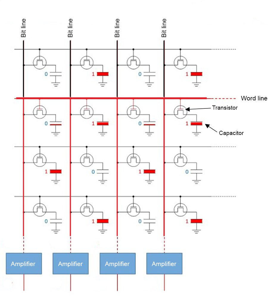
FIGURE 12.2: Sixteen DRAM memory cells each representing a bit of information for computational storage, reading, or writing. To read the binary word line 0101... in row two of the circuit, binary signals are sent down the bit lines to sense amplifiers.
Example 12.3 \(\text{}\)
One can get the total RAM on a Windows machine using the cmd command systeminfo.
Total Physical Memory: 32,564 MBI have around 32,000 megabytes = 32 gigabytes (Section 12.4) of RAM. One can obtain analogous results (in kilobytes) for Unix-likes using the BASH command free.
\(\blacksquare\)
Read-Only Memory (ROM): Primary memory (Fig 12.1) for software that is rarely changed (i.e., firmware). ROM includes functions for initializing hardware components and loading the operating system.
Motherboard: A circuit board physically connecting computer components including the CPU, RAM, ROM, and memory disk drives.
Disk drives: including CD, DVD, hard disk (HDD), and solid state disk (SSD) are used for secondary memory (Fig 12.1). That is, memory that is not directly accessible from the CPU. Secondary memory can be accessed or retrieved even if the computer is off. Secondary memory is also non-volatile and thus can be used to store data and programs for extended periods. User files and application software (like R) are generally stored on HDDs or SSDs. Flash memory, which uses modified metal–oxide–semiconductor field-effect transistors (MOSFETs), is typically used on USB and SSD devices to provide secondary memory that can be erased and reprogrammed. Flash memory can also be used in RAM applications.
Basic Input Output System (BIOS): Basic boot (startup) and power management firmware (software that provides low level control for computer hardware). Although historically, BIOS was stored on a physical ROM chip. It is now stored on a flash memory chip that can be updated.
12.2 Base-2 and Base-10
To understand computer processes, it is important to distinguish base-2 (binary) and base-10 (decimal) numerical systems. In both cases, the base refers to the number of unique digits. Thus, base-2 systems can have two unique digits, commonly \(0\) and \(1\), and the base-10 system has 10 unique digits: \(0,1,2,3,4,5,6,7,8,9\). The latter –more widely used system– probably arose because we have ten fingers for counting184. A radix (commonly a decimal symbol) is used to distinguish the integer part of a number from its fractional part (Fig 12.3). The radix convention is used by both base-2 and base-10 systems.
Example 12.4 \(\text{}\)
For example, the decimal number \(4\frac{3}{4}\), has integer component \(4\) and fractional component \(\frac{3}{4}\), and can be expressed as \(4.75\). We will soon learn that the binary equivalent of \(4\frac{3}{4}\) is 100.110. This expression has integer component 100 and fractional component 0.110 (Courier font is used here to emphasize the frequent use of binary expressions in computer processes).
\(\blacksquare\)
Traditionally, a base-10 number could only be expressed as a rational fraction whose denominator was a power of ten (Fig 12.3). However, the decimal system can be extended to any real number, by allowing a conceptual infinite sequence of digits following the radix (Wikipedia 2025h).
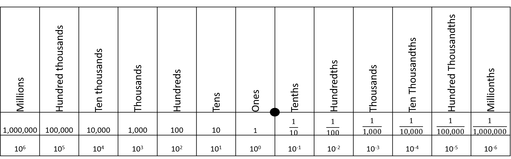
FIGURE 12.3: A decimal place value chart. A radix (decimal) is placed between the ones and thenths columns to distinguish decimal number components greater than one (to the left), and components less than one but greater than zero (to the right).
12.3 Scientific Notation
Under scientific notation, the integer component of a number is expressed with a single digit, and the remainder of the number is summarized by a fractional component, multiplied by a base raised to an integer. Scientific notation provides a consistent means of measuring the precision of a numeric expression.
Example 12.5 \(\text{}\)
The decimal number \(1245.42\) would be expressed, using scientific notation, as \(1.24542 \times 10^3\). The exponent value, \(3\), reflects the fact that the radix has been moved three digits to the left. The notated expression has a precision of six digits because \(1.24542\) contains six significant digits. In theory, one could approximate \(1245.42\) using \(1.2454 \times 10^3\), with the loss of one digit of precision.
Similarly, the decimal number \(0.00279\) would be expressed as \(2.79 \times 10^{-3}\), given a precision of three digits. The exponent value, \(-3\), reflects the fact that the radix has been moved three digits to the right.
\(\blacksquare\)
Example 12.6 \(\text{}\)
As noted in Example 12.4, the binary expression for \(4\frac{3}{4}\) is 100.110.
In binary scientific notation, expressed to six digits of precision, we have: 1.00110 \(\times\) 210. The exponent 10 is used because the radix has been moved two positions to the left, and binary expression for \(2\) is 10.
\(\blacksquare\)
12.4 Bits and Bytes
Computers are designed around bits and bytes. A bit is a binary (base-2) unit of digital information. Specifically, a bit will represent a 0 or a 1. This convention occurs because computer systems typically use electronic circuits that exist in only one of two states, on or off. For instance, DRAM memory cells (Fig 12.2) convert electrical low and high voltages into binary 0 and 1 responses, respectively. These signals allow the reading, writing, and storage of data. Although bits are used by all software in all conventional computer operating systems, these mechanisms are easily revealed in R.
For historical reasons, bits are generally counted in units of bytes. A byte equals eight bits. There are two major systems for counting bytes. The most common uses powers of 10, allowing implementation of SI prefixes (i.e., kilo = \(10^3 = 1000\), mega = \(10^6\) = \(1000^2\), giga = \(10^9\) = \(1000^3\), etc.) (Table 12.1). A computer hard drive with 1 gigabyte (1 billion bytes) of memory will have \(1 \times 10^9\) bytes = \(8 \times 10^9\) bits of memory. A second system, used frequently to describe RAM, uses a base-2 approach, with the conventions: \(2^{10} = 1024\) = kibi, \(2^{20} = 1024^2\) = mebi, \(2^{20} = 1024^2\) = gibi, etc. (Table 12.1).
| Base-10 | Base-2 | ||
|---|---|---|---|
| Bytes | Name | Bytes | Name (IEC) |
| \(1000\) | kB (kilobyte) | \(1024\) | KiB (kibibyte) |
| \(1000^2\) | MB (megabyte) | \(1024^2\) | MiB (mebibyte) |
| \(1000^3\) | GB (gigabyte) | \(1024^3\) | GiB (gibibyte) |
| \(1000^4\) | TB (terabyte) | \(1024^4\) | TiB (tebibyte) |
| \(1000^5\) | PB (petabyte) | \(1024^5\) | PeB (pebibyte) |
With a single bit we can describe only \(2^1 = 2\) distinct digital objects. These will be an entity represented by a 0, and an entity represented by a 1. It follows that \(2^2 = 4\) distinct objects can be described with two bits, \(2^3 = 8\) entities can be described with three bits, and so on185.
12.5 Decimal to Binary
We count to ten in binary using: 0 = 0, 1 = 1, 10 = 2, 11 = 3, 100 = 4, 101 = 5, 110 = 6, 111 = 7, 1000 = 8, 1001 = 9, and 1010 = 10. Thus, we require four bits to count to ten. Note that the binary sequences for all positive integers greater than or equal to one, start with one.
12.5.1 Positive Integers
We can obtain the binary expression of the integer part of any decimal number by iteratively performing integer division by two, and cataloging each modulus. The iterations are stopped when a quotient of one is reached. The modulus sequence is read from right to left, going from lower to higher powers of base 2, begining at the radix. If the whole number of interest is greater than one (i.e., the whole number is not 0 or 1) we place a one in front of the reversed sequence, because all binary sequences for numbers greater than or equal to one must start with one.
Example 12.7 \(\text{}\)
Consider the number 23:
\[ \begin{aligned} &\text{Modulus (remainder) }& 1& & 1& & 1& & 0&\\ &\text{Integer quotient } & 23/2 = 11& & 11/2 = 5& & 5/2 = 2& & 2/2 = 1& \end{aligned} \]
The reversed sequence is 0111. We place a one in front to get the binary representation for 23: 10111. The function dec2bin() from asbio does the work for us:
[1] 10111\(\blacksquare\)
12.5.2 Positive Fractions
The fractional part of a decimal number can be converted to binary in a similar fashion.
- To identify the fractional expression as a non integer, start the binary sequence with
0.(a zero followed by a decimal symbol). - Double the fraction to be converted, and record a
1if the product is \(\ge 1\), and record a0otherwise. - For subsequent binary digits, multiply two by the fractional part of the previous multiplication. If the product is \(\ge 1\), record a
1. If not, record a0.
Example 12.8 \(\text{}\)
Consider the fraction \(\frac{1}{4}\). We have:
\[ \begin{aligned} &\text{Binary outcome}& 0 && 1\\ &\text{Product} & 1/4 \times 2 = 1/2 < 1 && 1/2 \times 2 = 1\ge 1 \\ &\text{Binary outcome}& 0 && 0\\ &\text{Product} & 0 \times 2 = 0 < 1 && 0 \times 2 = 0 < 1 \end{aligned} \]
\(\blacksquare\)
We have a clear repeating sequence of zeroes, due to a product of two in the second step. This allows us to stop the growth of the binary expression. For fractions, the binary sequence is read from left to right (starting at the zero to the left of the radix). Thus, the binary expression for \(\frac{1}{4}\) is 0.01 .
dec2bin(0.25)[1] 0.0112.5.3 Negative numbers
Several methods have been developed for converting negative decimal numbers to binary. These generally require use of an extra sign bit as the leftmost (leading) bit, to indicate the number’s sign. The frequently used two’s complement procedure has three steps.
- Begin with the binary expression for the positive decimal number, and place
0in front of the expression to indicate the sign of the expression is positive. If one wishes to simply express a positive decimal number under two’s complement, then the conversion process ends here. - To obtain the additive inverse of a two’s complement expression (e.g., to obtain a negative number from a positive number) invert all the bits. That is, convert all
1bits to0bits, and vice versa. - Add
1to the rightmost digit in the inverted expression. In the case of a number with fractional components, a number less than 1 will actually be added. For example, adding a one to the last digit of1.01results in1.10, which is an increase of 0.25 in decimal units.
Example 12.9 \(\text{}\)
The binary expression for the decimal number 23 is 10111 (Example 12.7). To obtain the binary expression for -23 under two’s complement, one should complete the following steps:
- Place a
0in front of the10111to obtain the two’s complement expression for +23:010111. - Convert
1bits to0bits, and vice versa, to obtain:101000. - Add a one (in binary) to the rightmost digit to obtain:
101001. Note that if the last two digits were01, before adding a one, then adding one would result in the last two digits being10. That is,01+1=10.
To check the result, I can useasbio::dec2bin.twos():
dec2bin.twos(-23)[1] 101001\(\blacksquare\)
12.6 Binary to Decimal
Numeric outcomes from an underling base framework (e.g., binary, decimal) can be considered as a dot product (the sum of the element-wise multiplication of two numeric vectors). This can be represented with an equation based on Horner’s method (Horner 1815).
\[\begin{equation} \sum_{\kappa=\max(\kappa)}^{\min(\kappa)}\alpha\beta^\kappa \tag{12.1} \end{equation}\]
The term \(\alpha\) represents a vector of digits known as the significand or mantissa. Let \(a\) represent the individual digits comprising \(\alpha\), then \(\alpha = aaa \ldots\), where \(a \in \{0,1,\ldots, 9\}\), under a decimal framework, and \(a \in \{0,1\}\), under a binary format. The significand will be equivalent to the underlying (binary or decimal) numeric expression, except that the radix will be omitted.
The \(\beta\) term is the modifying base. For decimal expressions, \(\beta = 10\), and for binary expressions, \(\beta = 2\).
The \(\kappa\) term in Eq (12.1) is called (appropriately) the exponent. It will be a vector of the same length as \(\alpha\). The maximum and minimum values of \(\kappa\) are determined by counting the number of significant digits with respect to the radix in the underling numeric expression. The counting process for \(\kappa\) actually starts at the first digit to the left of the radix for both decimal (Fig 12.3) and binary expressions (Fig 12.4). Positive \(\kappa\) values (if any) occur for the integer components of the underlying numeric expression, with counts conducted right-to-left, and negative \(\kappa\) values (if any) result from left-to-right counts with respect to fractional component of the expression. Let \(x\) represent the individual digits comprising \(\kappa\), then, \(\kappa = \max(x), \max(x)-1, \max(x)-2, \ldots, \min(x)\), where \(x \in \mathbb{Z}\), and \(\mathbb{Z}\) represents all possible integers (positive, negative, and zero).
Eq (12.1) provides a generalized framework for obtaining decimal expressions from integer and fractional notations, including scientific notation, under different base formats. The potential movability of the radix in this context has resulted in the name floating point arithmetic.
Example 12.10 \(\text{}\)
For the decimal number \(1245.42\). We have the significand \(\alpha =\) 124542, \(\beta = 10\), and the maximum and minimum values of \(\kappa\) are 3 and -2, respectively. Thus, we have:
\[ \sum_{i = 3}^{-2} \alpha_i \times 10^i = \]
\[ \begin{aligned} &1 \times 10^3 + 2 \times 10^2 + 4 \times 10^1 + 5 \times 10^0 + 4 \times 10^{-1} + 2 \times 10^{-2}= \\ &1000 \hspace{.22in}+ 200 \hspace{.315in}+ 40 \hspace{.42in}+ 5 \hspace{.51in}+ 0.4 \hspace{.465in}+ 0.02 \hspace{.36in}= 1245.42 \end{aligned} \]
\(\blacksquare\)
Binary examples of Eq (12.1) are considered in the next two sections.
12.6.1 Positive Integers
The addition of a binary digit (i.e., a bit) represents a doubling of information storage. For instance, as we increase from two bits to three bits, the number of describable integers increases from four (integers 0 to 3) to eight (integers 0 to 7).
For positive integers the entirety of a corresponding binary expression will be to the left of the radix point (Fig 12.4). Thus, the minimum value of \(\kappa\) will be zero and the maximum value of \(\kappa\) will be the number of digits (bits) in the binary expression, minus one.
When applying Equation (12.1) to find the decimal integers represented by a single binary bit, we multiply the binary digit value, 0 or 1, by the power of two it represents in \(\kappa\). Because the single bit signature would occur at the right-most address to the left of the radix, the value of exponent would be 0 (Fig 12.4). That is, when considering Eq. (12.1), \(\min(\kappa)\) = \(\max(\kappa) = 0\).
If a single bit equals 0 we have:
\[0 \times 2^0 = 0,\]
and if the single bit equals 1 we have:
\[1 \times 2^0 = 1.\]
Accordingly, to find the decimal version of a set of binary values, we take the sum of the products of the binary digits and their corresponding (decreasing) powers of base 2.

FIGURE 12.4: Conceptualization of binary to decimal conversion of a positive integer and positive fraction, as given in Eq (12.1).
Example 12.11 \(\text{}\)
Because it doesn’t have a fractional component, the binary expression 010101 will be the same as the significand, \(\alpha\), The maximum and minimum values of \(\kappa\) will be 5 and 0, respectively. Because this is a binary expression, \(\beta = 2\). Thus, we have the following framework for Eq (12.1):
\[ \sum_{i = 5}^{0} \alpha_i \times 2^i = \]
\[ \begin{aligned} &(0 \times 2^5) + (1 \times 2^4) + \\ &(0 \times 2^3) + (1 \times 2^2) + \\ &(0 \times 2^1) + (1 \times 2^0) = \\ &0 + 16 + 0 + 4 + 0 + 1 = 21.\\ \end{aligned} \]
The function bin2dec in asbio does the calculation for us.
bin2dec(010101)[1] 21\(\blacksquare\)
12.6.2 Positive Fractions
For positive fractions, values of the \(\kappa\) exponent will decrease by minus one as bits increase by one (Fig 12.4). Thus, to obtain decimal fractions from binary fractions we multiply a bit’s binary value by decreasing negative powers of base two, starting at 0, and find the sum, as shown in Eq (12.1).
Example 12.12 \(\text{}\)
For the binary value 0.01, we have the significand \(\alpha\) = 001.
\[ \sum_{i = 0}^{-2} \alpha_i \times 2^i = \] \[(0 \times 2^0) + (0 \times 2^{-1}) + (1 \times 2^{-2}) = 0.25\]
bin2dec(0.01)[1] 0.25\(\blacksquare\)
Example 12.13 \(\text{}\)
To consider a decimal number with both integer and fractional components, recall that the decimal number 23.25 has the decimal expression 10111.01 (Example 12.5). Using 1011101 as the significand in Eq (12.1) we have:
\[ \sum_{i = 4}^{-2} \alpha_i \times 2^i = \]
\[ \begin{aligned} (1 \times 2^4) + (0 \times 2^{3}) + (1 \times 2^{2}) + (1 \times 2^{1}) + \\ (1 \times 2^{0}) + (0 \times 2^{-1}) + (1 \times 2^{-2}) = 23.25 \end{aligned} \]
\(\blacksquare\)
12.6.2.1 Terminality
Most decimal fractions will not have a clear terminal binary sequence. In this case, a binary representation of a decimal fraction with a finite number of digits will not exist. This results in mere binary approximations of decimal numbers (Goldberg 1991). For instance, the 10 bit binary expression of \(\frac{1}{10}\) is
dec2bin(0.1)[1] 0.0001100110But translating this back to decimal we find:
bin2dec(0.0001100110)[1] 0.099609We can increase the number of bits in the binary expression,
dec2bin(0.1, max.bits = 14)[1] 0.00011001100110This increases precision, but the decimal approximation remains imperfect.
[1] 0.0999755859375
1/10[1] 0.10000000000000000555Note that these imperfect conversions are the actual results of the division \(\frac{1}{10}\) for all software on all current conventional computers (not just R)!
It may seem surprising that rational fractions like \(\frac{1}{10}\) may have non-terminating binary expressions. Terminality, however, will only occur for a decimal fraction if a product of 2 results from the successive multiplication steps described in Section 12.5.2. This product does not occur for \(\frac{1}{10}\).
Lack of terminality for binary expressions prompts the need for quantifying bias and imprecision in computers systems.
12.6.3 Negative numbers
We can obtain negative decimal numbers, by assuming a two’s complement format, and applying Eq (12.1).
Example 12.14 \(\text{}\)
The two’s complement binary representation of -23 is 101001, with the leading bit serving as a sign bit (Example 12.14). Thus, we have:
\[
\begin{aligned}
-(1 \times 2^5) + (0 \times 2^{4}) + (1 \times 2^{3}) +\\ (0 \times 2^{2}) + (0 \times 2^{1}) + (1 \times 2^{0}) =\\ -23.
\end{aligned}
\]
We check our answer in R after specifying sign.bit = TRUE in bin2dec(). This command tells the function that the leading bit is a sign bit.
bin2dec(101001, sign.bit = T)[1] -23\(\blacksquare\)
12.7 Double Precision
In most programs, on most computers, numeric outcomes are stored as 32 bits (i.e., 4 bytes) or as 64 bits (8 bytes) of information186.
The 64 bit IEEE 754 double-precision binary floating-point format (binary64) (Kahan 1996), used by R allows high precision storage of both positive and negative integers and their fractional components. Under binary64, one bit is allocated to the sign of the stored datum, 52 bits are given to the significand, and 11 bits are given to the exponent (Fig 12.5).
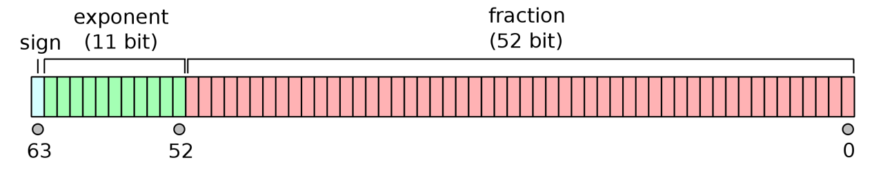
FIGURE 12.5: The IEEE 754 double-precision binary floating-point format. Figure from https://commons.wikimedia.org/w/index.php?curid=3595583.
The binary64 format can be expressed as a more complex form of Eq (12.1) .
\[\begin{equation} (-1)^{\text{sign}}\left(1 + \sum_{i=1}^{52} b_{52-i} 2^{-i} \right)\times 2^{E-1023} \tag{12.2} \end{equation}\]
Eq (12.2) gives the assumed decimal value for a 64-bit double-precision binary datum with exponent bias. In correspondence with Fig 12.5, the equation is the product of three components. .
The \(\text{sign}\) term in Eq (12.2) corresponds to the sign bit in Fig 12.5. That is, \(\text{sign} \in \{0,1\}\), resulting in potential outcomes \((-1)^{0} = 1\) and \((-1)^{1} = -1\).
The expression \(1 + \sum_{i=1}^{52} b_{52-i} 2^{-i}\) in (12.2) represents the 52 bit significand in Fig 12.5, and results in a scientifically notated fractional component of a numeric datum under an assumed base two format. Specifically, the notation will have an implicit leading one, i.e., \(1.\), and numbers following the radix will be the result of \(\sum_{i=1}^{52} b_{52-i} 2^{-i}\), which is a dot product of the 52 individual bit outcomes in the significand –that is, \(b_{52-i} \in \{0,1\}\) for \(i = 1,2,3,\dots, 52\)– and a vector resulting from base-2 raised to the sequence \(-1\) to \(-52\).
The expression \(2^{E-1023}\) in (12.2) corresponds to the exponent component of Fig 12.5), and allows binary64 to represent a wide range of numeric outcomes. \(E\) itself is a decimal translation of the 11 bit exponent, with minimum value:
bin2dec("000000000000")[1] 0-
and maximum value:
bin2dec("11111111111")[1] 2047-
Equation (12.2) has an excess-1023 offset binary format. This allows representation of both positive and negative exponents (with a pivot around 1023) without memory allocation for an additional sign bit. The pivot point of 1023 is used because it is approximately halfway between the minimum and maximum values of an 11 bit expression. Thus, values of E less than 1023 will result in a positive exponent (allowing the exponential expression of large magnitude positive and negative numbers), and values of E greater than 1023 will result in a negative exponent (allowing the expression of very small fractions).
Example 12.15 \(\text{}\)
The function bit64() below is taken from the documentation for the base function numToBits()187. The function distinguishes:
- The single bit defining the sign of the number (
0= positive,1= negative). - The 11 bit exponent.
- A 52 bit significand (53 bits with the implicit leading
1).
bit64 <- function(x)
  noquote(vapply(as.double(x),
    function(x) {
      b <- substr(
        as.character(rev(numToBits(x))), 2L, 2L)
      paste0(c(b[1L], " ", b[2:12], " | ", b[13:64]),
             collapse = "")}, "")
)- On Line 2, the script
noquote(vapply(as.double(x),initiates the functionvapply()which will return a vector of results given the application of some function (specified as the second argument invapply()) to some object (defined in the first argument ofvapply()). The first argument ofvapply()here is a double precision object coerced from the sole argument,xrequired bybit64(). The ultimate output frombit64()is a character string. The functionnoquote()will remove quotes from the string when the results are printed. - Lines 3-6 define the function to be run by
vapply()in it its second argument. That is, these lines are contained in the call tovapply().- The script on Line 4:
substr(as.character(rev(numToBits(x))), 2L, 2L)obtains 64 packets, each comprised of two memory bits, representing the decimal number inx, usingnumToBits(x), then reverses those packets withrev(), then converts those packets to strings withas.character()and finally retrieves the second digits from each packet withsubstr(., 2L, 2L). - On Lines 5-6 the character vector of length 64,
b, resulting from processes in Line 4, is subset into the sign bitb[1L], the exponentb[2:12], and the significandb[13:64]components of the 64 bit representation.
- The script on Line 4:
Here is the double precision representation of \(\frac{1}{3}\)
bit64(1/3)[1] 0 01111111101 | 0101010101010101010101010101010101010101010101010101We see this follows the form of Eq (12.2). The exponent 01111111101 represents the decimal number 1021:
bin2dec(01111111101)[1] 1021And one plus the dot product of the significand and a vector resulting from base-2 raised to the sequence -1 to -52, multiplied by \(2^{1021 - 1023}\), is:
sigd <- strsplit(
  "0101010101010101010101010101010101010101010101010101", NULL)
sigd <- as.numeric(unlist(sigd))
base2 <- 2^(-1:-52)
(1 + sum(sigd * base2)) * 2^-2
[1] 0.3333333That is, we have:
\[ \begin{aligned} value &= (-1)^{\text{sign}}\left(1 + \sum_{i=1}^{52} b_{52-i} 2^{-i} \right)\times 2^{E-1023}\\ &= -1^{0} \times (1 + 2^{-2} + 2^{-4} + \dots + 2^{-52}) \times 2^{1021-1023}\\ &\approx 1.33\bar{3} \times 2^{-2}\\ &\approx \frac{1}{3} \end{aligned} \]
\(\blacksquare\)
The 11 bit width of the double precision exponent component in Eq (12.2) allows the expression of numbers between \(2^{-1022} \approx 2.0 \times 10^{-308}\) and \(2^{1023} \approx 1.0 \times 10^{308}\)
We see that the lower numerical limit for in R (ver 4.5.3) is somewhere between:
-1.7 * 10^308[1] -1.7e+308and
-1.8 * 10^308[1] -InfAnd the upper limit is between:
1.8 * 10^307[1] 1.8e+307and
1.8 * 10^308[1] InfBetween these extremes, binary representations will have 15–17 decimal digit precision (because \(\log_{10} (2^{53}) \approx 16\)). This is clearly demonstrated in R, wherein imprecision problems with non-terminal fractions become evident for decimal numbers with more than 16 displayed decimal digits.
options(digits = 18)
1/3
[1] 0.333333333333333315The so-called subnormal representation188 compromises precision, but allows allows fractional representations approaching \(5 \times 10^{-324}\). This approach is used by R, whose smallest represented fraction is between:
5.0 * 10^-323[1] 4.941e-323and
5.0 * 10^-324[1] 0Reflecting most software, integers in R are stored (exactly) in a signed four byte (32 bit) format. Given that one bit is used to represent the sign of the integer, and a placeholder is needed for the outcome 0, the current minimum and maximum value for an integer in R are \(-2^{31} = -2,147,483,648\) and \(2^{31} -1 = 2,147,483,647\), respectively.
.Machine$integer.max[1] 214748364712.8 Hexadecimal
After base 2, hexadecimal (base 16) is the most common numerical system used in computing (Haddock and Dunn 2011). The system uses the hexes A-F or a-f to represent decimal numbers 10-15. Thus, in order, the sixteen unique hexes are: 0,1,2,3,4,5,6,7,8,9,A,B,C,D,E,F. To indicate that the hexadecimal system is being used by a computer, hex values are often written with a preceding 0 or 0x. Thus, 0F, 0xF could be used to represent the hex F, the 16th hex, which corresponds to decimal number 15, and the binary representation 1111. Ultimately, hexidecimal encoding must be translated to binary machine code for a computer to understand it.
The subscripts 10, 2, and 16 are often used to distinguish decimal, binary and hexadecimal expressions, respectively. For instance, 1510 = 11112 = F16. One would reuse hexes for numbers larger than 15, just as one would reuse decimal digits to represent numbers larger than 9. For instance, 1016 = 1610, 2016 = 3210, 3016 = 4810, \(\dots\), A016 = 16010, and so on.
Example 12.16 \(\text{}\)
Here I use asbio::dec2bin() and base::as.hexmode() to obtain binary and hexadecimal representations of the first twenty-one decimal numbers, including zero.
dec <- 0:20
bin <- sapply(dec, dec2bin)
hex <- format(as.hexmode(dec))

data.frame(Decimal = dec, Binary = bin, Hexadecimal = hex)
Decimal Binary Hexadecimal
1 0 0 00
2 1 1 01
3 2 10 02
4 3 11 03
5 4 100 04
6 5 101 05
7 6 110 06
8 7 111 07
9 8 1000 08
10 9 1001 09
11 10 1010 0a
12 11 1011 0b
13 12 1100 0c
14 13 1101 0d
15 14 1110 0e
16 15 1111 0f
17 16 10000 10
18 17 10001 11
19 18 10010 12
20 19 10011 13
21 20 10100 14\(\blacksquare\)
An advantage of hexadecimal is that it allows simpler and more readable representations than binary. This is because the eight bits from one byte will correspond to exactly two hex digits. A sequence of two hex digits is often called a hexadecimal byte.
12.9 Binary and Hexadecimal Characters
Characters and other non-numeric data types can also be expressed in binary or hexadecimal. Computers distinguish overlapping binary encodings for different data types (e.g., numbers, characters, Boolean outcomes189, etc.) based on: 1) context (calculator and word processor programs will generally view binary inputs as numbers and characters, respectively), and 2) file headers and other metadata that distinguish data types. For example, the hexadecimal byte 0x57 is often used to denote a subsequent ASCII string (see below), whereas 0x23 can denote a subsequent 64 bit real number.
The American Standard Code for Information Interchange (ASCII) encoding system consists of \(2^7 = 128\) characters, and thus requires seven bits190. The Latin-1 system adds 128 characters to ASCII by requiring 8 bits (because \(2^8 = 256\)). The newer Unicode Transformation Format (UTF-8) system –the one generally used by R– can represent 1,112,064 code points, using between 1 to 4 bytes (8 to 32 bits), each codified as a hexadecimal byte (two hex digits) (Wikipedia 2025z). Currently, however, only 297,334 points have actually been assigned to characters191. The first 128 UTF-8 characters are the ASCII characters, and the first 256 UTF-8 characters are Latin-1, allowing back-comparability with those systems.
Example 12.17 \(\text{}\)
We can observe the process of binary character assignment in R using the functions as.raw(), rawToChar(), and rawToBits(). The base type raw (Section 2.4.8) is intended to hold raw byte information. Here is a list of the 128 ASCII characters.
  [1] "\001" "\002" "\003" "\004" "\005" "\006" "\a"   "\b"   "\t"   "\n"
 [11] "\v"   "\f"   "\r"   "\016" "\017" "\020" "\021" "\022" "\023" "\024"
 [21] "\025" "\026" "\027" "\030" "\031" "\032" "\033" "\034" "\035" "\036"
 [31] "\037" " "    "!"    "\""   "#"    "$"    "%"    "&"    "'"    "("
 [41] ")"    "*"    "+"    ","    "-"    "."    "/"    "0"    "1"    "2"
 [51] "3"    "4"    "5"    "6"    "7"    "8"    "9"    ":"    ";"    "<"
 [61] "="    ">"    "?"    "@"    "A"    "B"    "C"    "D"    "E"    "F"
 [71] "G"    "H"    "I"    "J"    "K"    "L"    "M"    "N"    "O"    "P"
 [81] "Q"    "R"    "S"    "T"    "U"    "V"    "W"    "X"    "Y"    "Z"
 [91] "["    "\\"   "]"    "^"    "_"    "`"    "a"    "b"    "c"    "d"
[101] "e"    "f"    "g"    "h"    "i"    "j"    "k"    "l"    "m"    "n"
[111] "o"    "p"    "q"    "r"    "s"    "t"    "u"    "v"    "w"    "x"
[121] "y"    "z"    "{"    "|"    "}"    "~"    "\177" "\x80"
Note that the exclamation point is character number 33. Its 16 bit binary code is:
[1] 01 00 00 00 00 01 00 00From the output above, codes 1-31 and 127-128 are non-printable control characters. For instance, recall (Section 4.3.3.4) that \t (ASCII code 9) represents the tab key, Tab, and \n (ASCII code 10) represents new line. Thus, there are only 128 - 33 = 95 printable ASCII characters.
\(\blacksquare\)
Hexadecimal representations are usually used to denote Unicode characters by preceding the hex number with 0x00. The prefix \u00, however, is generally used in R192.
Example 12.18 \(\text{}\)
For instance, the explanation point $ is the 36th Unicode (and ASCII) character (Example 12.17). The 36th hex number (the hex representation of 3510) is 2416. So, the hexadecimal representation of $ is 0x0024. This can be verified with the base function intToUtf8().
intToUtf8("0x0024")[1] "$"We could use "\u0024" to obtain the Unicode character $ without using intToUtf8().
"\u0024"[1] "$"\(\blacksquare\)
12.10 R, the Internet, and the Web
For many R tasks, including administration of Shiny apps (Section 11.5.7.2) and data import from webpages (see Examples in Section 12.10.2), it will be useful to have a basic understanding the workings of the internet and the world wide web.
12.10.1 The Internet
From the perspective of computer science, a network is a group of interacting computers. A local area network (LAN) connects computational devices (computers, printers, etc.) within a specific area (a residence, building, etc.) to each other. Connections between network components are can be maintained thorough a combination of Ethernet cables, fiber-optic cables, and radio wave signals.
The internet is a global collection of networks, continually communicating with one another, via packets of information made up of digital bits, through a series of formal procedures193.
- The user is the individual accessing/using the internet.
- The client is a device (e.g., workstation, laptop tablet, phone) employed by the user to request information from servers.
- The server is a continuously running computer or network of computers that can potentially handle a wide variety of tasks, including website hosting, email management, and data sharing.
A host is a computer or other device connected to a network (including the internet). Thus, both clients and servers are hosts. Host-to-host connections require hardware, including modems, that connect local networks to the internet via an Internet Service Provider (ISP)194, and routers, which operate behind modems to direct data flows within and between networks, often wirelessly.
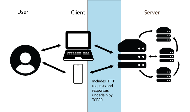
FIGURE 12.6: Conceptualization of internet information transfer. Figure uses vector art from https://www.flaticon.com (Md Tanvirul Haque), https://www.onlinewebfonts.com (licensed by CC BY 4.0 Amila Ruwan) and https://www.vecteezy.com.
Data transfer paths follow arrows in Fig 12.6 under a procedure called packet switching, in which data units called packets –underlain by data bits– are generated and transmitted. A packet will consist of a header, that contains handling information and the packet destination, and a payload (the transferred information). A single data stream may require multiple independent packets which must be reassembled when a data transfer is completed. This approach allows information subsets to be re-routed, preventing transfer roadblocks.
12.10.1.1 Protocols
Internet operations are made possible by a set of standards called the Internet Protocol Suite (IPS). These rules allow communications to work in the same way, regardless of variations in individual computer operating systems, internet software, and other constraints. The IPS can be described as an interacting process, made up of four layers (Braden 1989): the link layer, the internet layer, the transport layer, and the application layer (Fig 12.7). Facets of the IPS framework are described below (from bottom to top) with examples.
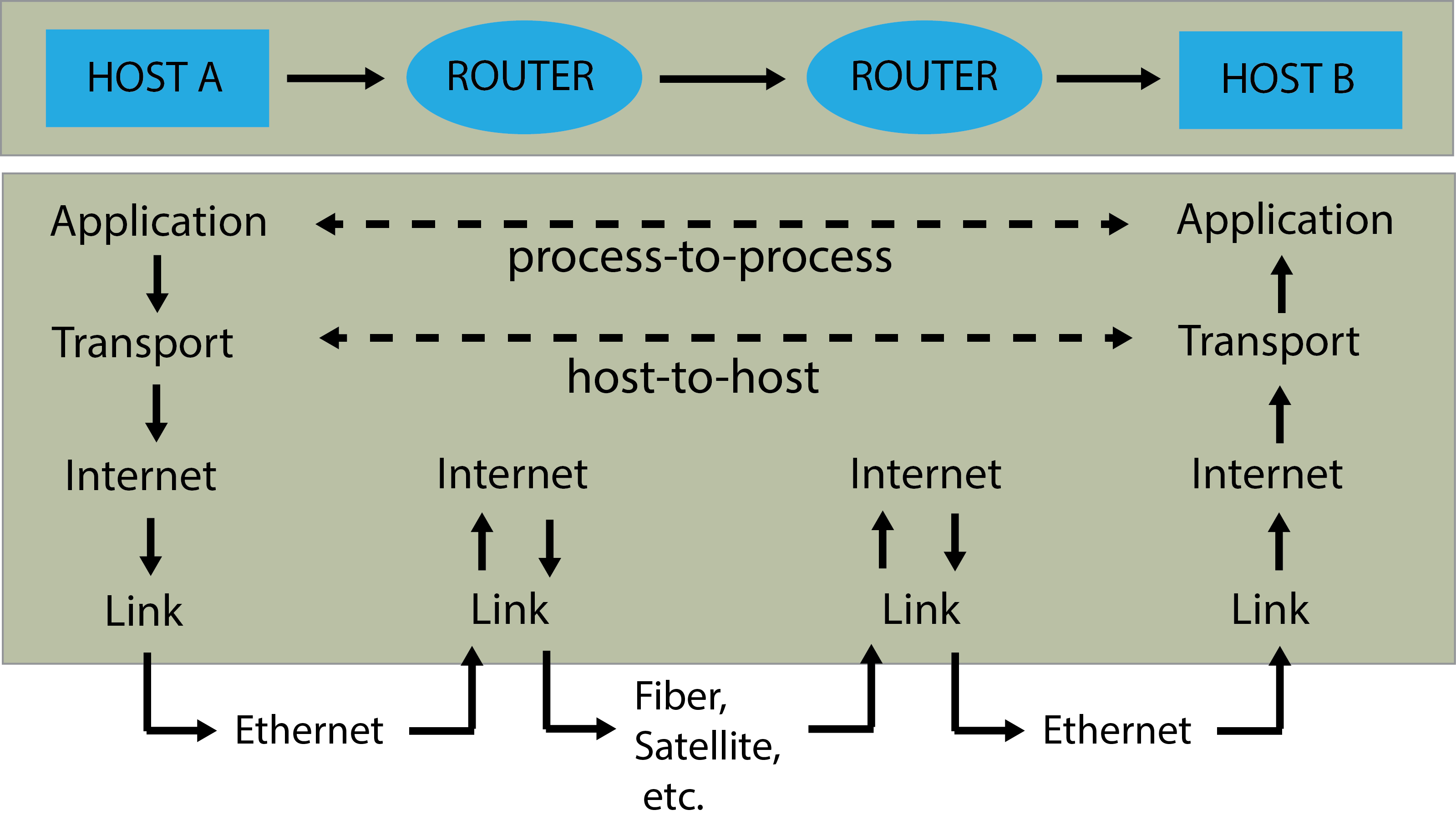
FIGURE 12.7: Flow of internet data. A shows two hosts (host A and host B) connected by a link between their routers, with information flowing from host A to host B. Applications at each host execute read and write operations through a data pipe. Figure and caption follow those at (https://en.wikipedia.org/wiki/Internet_protocol_suite)
The Link Layer operates only within the scope of the local network. Among other protocols, the layer adds or strips framing195 of data packets as they are transmitted or received, by a host respectively. Transmission and reception of packets occur through ethernet, fiber, and/or satellite connections (Fig 12.7).
-
The Internet Layer defines addressing and routing rules for sending data packets across network boundaries. The primary protocol of the internet layer is the Internet Protocol (IP) which includes standards for IP addresses, and packet path determination.
- An IP address is the primary system used to identify physical and virtual network locations. Public IP addresses are overseen by the non-profit Internet Corporation for Assigned Names and Numbers (ICANN). Specifically, ICANN allocates address blocks to Regional Internet Registrations (RIR)196, which assign them to ISPs. Router public IP addresses are ultimately assigned by ISPs. Thus, a public IP address is the location of your router from the perspective of the rest of the internet (Fig 12.8). A private IP address is assigned by your router and will be limited to your local network. IP addresses, both public and private, are currently defined using one of two numerical methods.
-
IPv4 uses 32 bits, and thus allows \(2^{32}\) distinguishable addresses. Address codes are generally displayed as four, eight bit numbers (decimal numbers from 0-255), separated by decimal symbols, or dashes. For example:
134.50.65.454. -
IPv6 uses 128 bits, and thus allows approximately \(3.403 \times 10^{38}\) distinguishable addresses. Address codes are based on up to eight hexadecimal representations, separated by colons, e.g.,
5649:ca30:a26b:2eba.
-
IPv4 uses 32 bits, and thus allows \(2^{32}\) distinguishable addresses. Address codes are generally displayed as four, eight bit numbers (decimal numbers from 0-255), separated by decimal symbols, or dashes. For example:
- An IP address is the primary system used to identify physical and virtual network locations. Public IP addresses are overseen by the non-profit Internet Corporation for Assigned Names and Numbers (ICANN). Specifically, ICANN allocates address blocks to Regional Internet Registrations (RIR)196, which assign them to ISPs. Router public IP addresses are ultimately assigned by ISPs. Thus, a public IP address is the location of your router from the perspective of the rest of the internet (Fig 12.8). A private IP address is assigned by your router and will be limited to your local network. IP addresses, both public and private, are currently defined using one of two numerical methods.
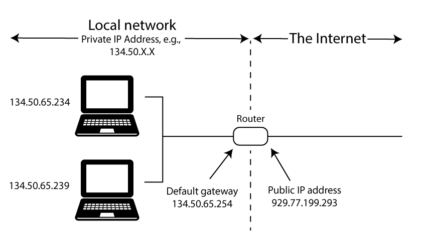
FIGURE 12.8: Conceptualization of public and private IP addresses. Figure uses vector art from https://www.vecteezy.com.
Example 12.19 \(\text{}\)
To get private IP information about my personal (Windows) computer I can use the command ipconfig in cmd.
Windows IP Configuration

Ethernet adapter Ethernet:
   Connection-specific DNS Suffix  . : isu.edu
   IPv4 Address. . . . . . . . . . . : 134.50.65.234

Ethernet adapter Ethernet 2:
   Media State . . . . . . . . . . . : Media disconnected

Ethernet adapter vEthernet (WSL (Hyper-V firewall)):
   IPv4 Address. . . . . . . . . . . : 172.27.160.1
There are three potential private network connections on my machine, the second of which is not being used. The first, with IPv4 address 134.50.65.234, allows connectivity to my Idaho State University network account. The third, with IPv4 address 172.27.160.1, allows connectivity to the Windows Subsystem for Linux (WSL) running on my machine. Analogous summaries for Unix-likes can be obtained using the BASH command ip addr.
\(\blacksquare\)
Example 12.20 \(\text{}\)
Locating a public (internet-facing) IP address requires use of external services. In the code below, I use the cmd command nslookup to access the website myip.opendns.com and the service resolver1.opendns, provided by OpenDNS (which is managed by Cisco).
The output 929.77.199.293 below is my (intentionally altered) public IP address (it is generally not a good idea to share your public IP address).
Non-authoritative answer:
Server:  dns.sse.cisco.com
Address:  929.77.199.293

Name:    myip.opendns.com
Address:  134.50.65.234
\(\blacksquare\)
- The Transport Layer consists of data channel protocols that allow host-to-host communication.
- User Datagram Prototcol (UDP): The simplest transport protocol, wherein packets are transferred as self-contained datagrams which allow connectionless (albeit potentially unreliable) communication.
- Transmission Control Protocol (TCP): An important transport-layer protocol that provides a “reliable, in-order, byte-stream service” to and from applications (Eddy 2022). Unlike UDP, TCP requires ordered data transfer of packets, retransmission of lost packets, error-free data transfer, and congestion/flow control of transmissions. Because TCP and IP were initially co-released, the entire internet protocol suite is often called TCP/IP.
-
Network ports are communication transfer endpoints that may map to particular protocols. A port is identified with a 16-bit unsigned integer. Thus, port numbers range from 0 to 65535. Ports 0-1023 are system ports used for common network processes. System ports include
22, Which prompts the secure Shell (SSH) login,25, which triggers the Simple Mail Transfer Protocol (SMTP) for use with email, and80and443indicate HTTP and HTTPS for standard web browsing and encrypted (secure) browsing, respectively. For details on these protocols see Application layer section below. An IP address conjoined with a port is called a network socket. In this case a host identifier (IP address) will be linked to a specific program or service endpoint (port).
Example 12.21 \(\text{}\)
Sockets will often be associated with IPS transport layer protocols, i.e., TCP and UDP. To identify active ports I could use the netstat shell command in cmd, Powershell, or BASH.
The options -an indicate that only active sockets should be listed, and these should be identified by their port number.
Here is a selection of output:
Active Connections

  Proto  Local Address          Foreign Address        State
  TCP    134.50.65.234:62595    35.190.43.134:443      ESTABLISHED
  TCP    134.50.65.234:63490    20.59.87.227:443       ESTABLISHED
  TCP    127.0.0.1:5354         0.0.0.0:0              LISTENING
  UDP    127.0.0.1:1900         *:*
  UDP    127.0.0.1:54291        127.0.0.1:54291
In the interest of brevity, I limit my interpretation here to the first line of output which concerns an established TCP connection between a local socket (private IP address = 134.50.65.234 (see Example 12.19), port = 62595) and a remote HTTPS socket (IP address = 35.190.43.134, port = 443). The port in the local socket, 62595, falls within the range of port numbers (49152 to 65535) that are not permanently assigned to specific services, but are allocated by the operating system as they are needed.
\(\blacksquare\)
- The Application layer includes protocols allowing the provision of user services and the exchange of information. The application layer is built atop connections established by lower-level protocols (i.e., the transport, internet, and link levels, Fig 12.7.).
- Hypertext Transfer Protocol (HTTP): Provides rules for content underlying the world wide web (Section 12.10.2). The protocol operates on a client-server basis, wherein a client will make requests to a server (Fig 12.6). HTTPS, a “secure” version of HTTP, is used by more than 85% of websites, including email servers.
- File Transfer Protocol Secure (FTPS): A protocol that provides a secure, less complex alternative to the older File Transfer Protocol (FTP). FTPS uses of an encryption tool called Transport Layer Security (TLS), which is also used by HTTPS.
-
Secure Shell Protocol (SSH): A protocol for operating network services securely over an unsecured network. The SSH can be called from Unix-like shells (e.g., BASH), as well as cmd and PowerShell, using the command
ssh.-
SSH File Transfer Protocol (SFTP): A protocol for transferring files to or from remote computers (including servers) with respect a local (client) computer, under an SSH connection. SFTP can be called from Unix-like shells as well as cmd and PowerShell using the command
sftp. Importantsftpcommands include:-
cd: change directories on remote machine. -
lcd: list files on local machine. -
ls: list files on remote machine. -
!ls: list files on local machine. -
get A B: downloadAfrom remote machine, and save it asBlocally. -
put A B: uploadAfrom local machine, and save it asBon remote machine. -
exit: closesftpconnection.
-
-
SSH File Transfer Protocol (SFTP): A protocol for transferring files to or from remote computers (including servers) with respect a local (client) computer, under an SSH connection. SFTP can be called from Unix-like shells as well as cmd and PowerShell using the command
Example 12.22 \(\text{}\)
I am an administrator for a server that contains a number of websites, including several that host Shiny apps (Section 11.5.7.2). Below I gain access to the server using the command ssh.
PS > ssh [email protected]
[email protected]'s password:
The server is a remote Linux computer operating with a 64 bit x86 CPU:
The IP address of the server is 172-31-35-117. The IPv4 range 172.16.0.0 – 172.31.255.255 is reserved for private networks, and is commonly used by AWS.
\(\blacksquare\)
Example 12.23 \(\text{}\)
Here I initiate SFTP to allow file transfer with the server.
PS > sftp [email protected]
[email protected]'s password:
Connected to kenaho.aws.cose.isu.edu.
sftp>
Note that we have a new command line prompt: sftp>. Here are first five items in current directory of my local machine:
Here are the contents of the working directory of the remote machine:
Here I transfer the file Amalgam-of-R.pdf from the local current directory to the working directory of the remote machine:
Uploading Amalgam-of-R.pdf to /home/ahoken/Amalgam-of-R.pdf
Amalgam-of-R.pdf              100%   36MB  30.2MB/s   00:01
Not bad, a 30.2MB/s upload rate.
\(\blacksquare\)
12.10.2 The Web
The world wide web (or simply web) allows internet access to media through dedicated web servers197 under the rules of HTTP or HTTPS. Websites are accessed by specifying a unique Uniform Resource Locator (URL) in a web browser program (e.g. Mozilla\(^{\circledR}\) Firefox, Apple\(^{\circledR}\) Safari). A URL will contain both a domain name, e.g., amalgamofr.org (amalgamofr and .org are considered second-level and top-level domain locations, respectively), along with the protocol (e.g.,https://), and, possibly, a path. The complete URL for the Ch 12 path in this book is: https://amalgamofr.org/ch12.
Domain names exist because they are easier to remember than IP addresses. However, they must be translated to binary, machine-readable IP addresses to allow communication between users and servers. This process is managed by Domain Name System (DNS) servers containing a copy of the master DNS database (slave DNS zone), which is updated many times a day.
The BASH tool curlallows one to transfer data to or from a server using URLs. Variants of curl also exist for cmd and PowerShell.
Example 12.24 \(\text{}\)
Here I download the simple mothur dataset from Example 9.15 using its URL, and redirect the data to the current working directory.
  % Total    % Received % Xferd  Average Speed   Time    Time     Time  Current
                                 Dload  Upload   Total   Spent    Left  Speed
  0     0    0     0    0     0      0      0 --:--:-- --:--:-- --:--:--     0100   551  100   551    0     0   1985      0 --:--:-- --:--:-- --:--:--  2025
\(\blacksquare\)
One can also use R functions directly, including download.file() and read.table() (if data are tabular), for internet downloads.
Example 12.25 \(\text{}\)
Here I download taxon.txt and redirect it to my working directory as the file taxon2.txt.
download.file("https://amalgamofr.org/taxon.txt", "taxon2.txt")\(\blacksquare\)
Cross-computer access is much easier on LANs, and to and from Unix-likes. Windows machines may require installation and configuration of tools like OpenSSH.
12.10.3 Internet Security
Security is a primary concern when moving information between clients and servers via file transfer protocols (Section 12.10.1.1), SQL database manipulation (Section 9.6), or other processes. Threats from internet interactions –including malware, phishing, and hacking– can be minimized through the use of:
Passwords are generally strings of characters used to confirm a users network identity. Passwords typically have a required minimum level of complexity (e.g., 12-16 characters, including special characters like:
~,!,@,#,$). Additionally, passwords often require pairing with a user name, and often serve as a mere sub-component to a multi-factor authentication procedure that may require transference of randomly generated sequences sent to a token or authenticator app.Encryption transforms information so that only authorized parties can decode it. Approaches include the TLS framework which protects HTTPS and FTPS using pseudo-random number key generators (Section 12.10.1.1), among other methods.
Anti-virus software prevents, detects, and removes malware (i.e., programs or code intended to damage a computer Wikipedia (2026c)). The status of installed Windows anti-virus products can be obtained with the cmd script:
displayName                productState
Sentinel Agent             266240
Trellix Endpoint Security  397312
Windows Defender 393472- The hexadecimal codes above indicate that the antivirus software is active and up to date.
- Firewalls monitor and control incoming and outgoing network traffic, based on security rules, including limiting network exchanges to particular IP addresses or ports. One can check the firewall status for a Windows computer using cmd:
Domain Profile Settings:
------------------------------------
State                                 ON

Private Profile Settings:
------------------------------------
State                                 ON

Public Profile Settings:
------------------------------------
State                                 ON
Domain, Private and Public firewall profiles constitute rule set that are increasingly strict, and are unique to windows. A potentially massive set of Windows firewall rules (not shown) for these components can be obtained with:
Unix-likes can obtain a computer’s firewall status using the BASH commands: sudo ufw status.
12.11 High Powered R
We have already learned a number of ways to improve the efficiency and capabilities of R. These include: 1) replacing loops with efficient functions like apply() whenever possible (Section 8.5.5), and 2) writing and calling compiled functions, including those written in C++ (Section 9.5), to drive processes in R.
In this section I briefly consider the use of R in parallel processing and high performance computing. This topic is particularly important to those managing highly iterative computational procedures or handling large biological datasets common in bioinformatic pipelines and spatiotemporal research.
12.11.1 Parallel Computing
In parallel computing, multiple computational processes are carried out simultaneously by assigning those processes (threads) to different CPUs or CPU cores. Parallel processing can be contrasted with conventional serial processing in which computational tasks are completed sequentially, one at a time. Parallel processes exist along a continuum from perfectly parallel, in which there is absolutely no dependency between tasks (allowing tasks to be completed simultaneously), to inherently serial (in which one task requires the result from another task). These extremes and their gradations may require programming adjustments for optimal efficiency.
Two general approaches for parallel processing in R are possible (Errickson 2024).
The socket method will open a new iteration of R on each core. This is done using private IP addresses on your computer, potentially triggering a system warning prompt. In this case, one should allow R to accept incoming connections.
The fork method copies the current
image()of R and runs it in other cores. Forking is programmatically simpler, and generally creates faster parallel processes than the socket method. Forking, however, is not currently supported in Windows.
The parallel base distribution package combines two older R packages: multicore and snow Tierney et al. (2021), to allow socket and fork processing.
The parallel package allows further optimization of the efficient apply family of functions (Section 4.1.1) with its parApply and mcapply functions. The functions parLapply(), parSapply(), and parApply() can be used as socket or fork analogs of lapply(), sapply(), and apply(), respectively, following creation of an appropriate cluster framework. The functions mclappy()and mcmapply() are fork analogs of lapply() and mapply(), and produce serial processes in Windows.
12.11.1.1 Socket processing
Socket processing requires four steps (Errickson 2024):
- Define a cluster with the desired number of cores/threads.
- Complete pre-processing steps (e.g., loading necessary packages) for each core.
- Run a parallel process, for instance, using
parApply(). - Under best practices, destroy the cluster.
Example 12.26 \(\text{}\)
It is generally not a good idea to use all available cores on a personal machine. Instead, Errickson (2024) recommends \(n/2\) as a good starting point. The parallel function detectCores() detects CPU cores198. Confirming our finding from Example 12.2, I have six available cores.
library(parallel)
detectCores()
[1] 6Here I create a cluster, cl, with three threads.
cl <- makeCluster(3)We can verify the functionality of the cluster by assigning a process using parallel::clusterEvalQ().
clusterEvalQ(cl, 2 + 2)Note the list output.
Here is a quick comparison of parallel and serial (using sapply()) run times for creating 3 datasets, each made up of \(10^8\) pseuduo-random standard normal observations.
# parallel (socket)
st1 <- system.time(clusterEvalQ(cl, rnorm(10^8)))

# serial
st2 <- system.time(
  replicate(3, rnorm(10^8)) # sapply() wrapper
  )

list(Parallel = st1,
Serial = st2)clusterEvalQ also provides a quick way to load packages (and their dependencies) for each core.
# package for linear mixed effect models
clusterEvalQ(cl, library(lme4)) [[1]]
[1] "lme4" "Matrix" "stats" "graphics"
[5] "grDevices" "utils" "datasets" "methods"
[9] "base"
[[2]]
[1] "lme4" "Matrix" "stats" "graphics"
[5] "grDevices" "utils" "datasets" "methods"
[9] "base"
[[3]]
[1] "lme4" "Matrix" "stats" "graphics"
[5] "grDevices" "utils" "datasets" "methods"
[9] "base" Here I use parLapply() and lappy() to create lists of length 10000, with each list component containing 10000 pseudo-random normal observations.
# parallel (socket)
st1 <- system.time(
  parLapply(cl, 1:10000, rnorm)
)
# serial (lapply)
st2 <- system.time(
  lapply(1:10000, rnorm)
)

list(Parallel = st1,
Serial = st2)When finished, one should destroy the cluster to stop background socket processes, and to prevent new processes from be slowed or delayed.
stopCluster(cl)Closing R will automatically close all cluster processes.
\(\blacksquare\)
12.11.1.2 Fork processing
As noted above, forking is not currently possible in native Windows OS. However, one can use WSL to implement the Linux kernel on a Windows machine, allowing fork processes. It very straightforward to run parallel forks (assuming you have a Unix-like OS).
Example 12.27 \(\text{}\)
To ensure that parallel processing is actually occurring we can run a simple time-consuming function through mclapply(). The function sum.then.wait() below calculates the sum of a number and itself for elements in a vector x, with a one second delay to start the process. If x has length \(n\), then, under serial processing, the system time should be approximately \(n\) seconds, because computation of the sum itself would take essentially no time. If \(n\) is less than or equal to the number of available cores, then we would expect the system time to be approximately one second, because the function would start for all elements, simultaneously.
Here I access WSL and open R in Linux.
\(\blacksquare\)
Example 12.28 \(\text{}\)
Here I create a million datasets of size 10, and use a fork to calculate the mean of each. This exercise is repeated, in higher powered contexts, in Examples 12.30 and 12.31.
\(\blacksquare\)
12.11.2 HPC clusters and R
A cluster is a set of computers (nodes) that work together, often through parallel processing, as a single high performance unit. My current employer (Idaho State University) is allowed access to High Performance Computing (HPC) clusters located at the Idaho National Laboratory, a nuclear energy research facility. Following coordination with a system administrator, these supercomputers can be accessed through a remote Virtual Machine (VM) server, and interfaced using a BASH terminal embedded in a webpage. The INL Lemhi supercomputer (named after a nearby Idaho mountain range) is a “relatively small” cluster underlain by 504 nodes, with dual 20 core CPUs at each node. Thus, in total, the cluster contains 504 \(\times\) 2 \(\times\) 20 = 20,160 cores. Each node in the cluster contains 192 MB of RAM and 94.5 TB of total memory. The nodes use the Rocky Linux operating system, which is designed to be extremely stable, with 10 years of support for OS versions.
Example 12.29 \(\text{}\)
Gaining access to Lemhi requires a login process managed by a web GUI. After accessing Lemhi, system specifications can be obtained using BASH commands like lspcu (which describes CPU architecture) and nproc (which counts the number of available core processing units).
Last login: Tue Feb 10 10:25:00 2026

(base) ahoken.isu@lemhi ~ > lscpu | grep "Model name"
Model name:          Intel(R) Xeon(R) Gold 6148 CPU @ 2.40GHz

(base) ahoken.isu@lemhi ~ > nproc
40
We see that each node (computer) in the Lemhi cluster contains 40 cores.
The Lemhi cluster is set up to use Miniconda as a software distribution source, with conda as the package manager (see Sections 9.7.2 and 9.7.3). To use R, I first create a new conda environment to house R and the R packages I want to use, with the conda utility create.
The create option -n allows the specification of a user-supplied environment name, in this case, r-env.
Here I list my environments
# conda environments:
#
# * -> active
# + -> frozen
base         /lfs/ahoken.isu/miniconda3
r-env   *    /lfs/ahoken.isu/miniconda3/envs/r-env
I activate r-env using the conda utility activate.
(r-env) ahoken.isu@lemhi ~ >I can install R (and roughly 200 “essential” R packages) using conda install.
I can now open Rterm (a GUI-less R-terminal) by simply typing R at the command line.
\(\blacksquare\)
12.11.2.1 Slurm –Single Compute Node
Most HPC networks will initially deliver one to a head node that will be sub-optimal for high performance computing. Apportioning nodes in HPCs is often handled by an open-source job scheduler called Slurm (Simple Linux Utility for Resource Management).
Example 12.30 \(\text{}\)
Using Slurm, I can obtain exclusive access to a single compute node for one hour with:
Of primary importance is the Slurm command srun, which I run with options --nodes=1, --exclusive, and --time=01:00:00 (the lack of spaces is important). The option --pty bash -i opens a interactive BASH pseudo-terminal (in this case, terminal 0001).
To test the capabilities of R in this setting, we can activate the r-env environment (which contains R) and start R.
Here I redo Example 12.28, with much faster results.
library(parallel)

rep <- replicate(1000000, rnorm(10), simplify = FALSE)

# parallel (fork)
st1 <- system.time(
  system.time(mclapply(rep, mean, mc.cores = 30))
)
# serial (lapply)
st2 <- system.time(
  save2 <- lapply(rep, mean)
)

list(Parallel = st1,
     Serial = st2)
$Parallel
user system elapsed
6.711 5.949 0.696
$Serial
user system elapsed
3.840 0.036 3.884 \(\blacksquare\)
12.11.2.2 Slurm Batch –Multiple Nodes
The parallel package was created primarily for parallel computing on a single node. Multi-node applications are possible, however, using either sockets or forks. Notably, R currently allows “only” 125 open connections, limiting the number of usable cores, across nodes.
Multi-node HPC procedures are generally executed from a batch shell script, initiated by a shebang (Section 9.2.8). The script specifies Slurm parameters (i.e., number of nodes, number of cores, etc.), along with other shell commands, including calls to external source code. For example, the R source code file foo.R could be called from BASH using R CMD BATCH foo.R or Rscript foo.R (Example 9.19)..
Example 12.31 \(\text{}\)
Below I create an R script that repeats Example 12.30. I will save the script as a text file named test1.R in my home directory on the Lemhi HPC.
### test1.R
cl <- parallel::makeForkCluster(nnodes = 120)

rep <- replicate(1000000, rnorm(10), simplify = FALSE)

system.time(parLapply(cl, rep, mean))
parallel::stopCluster(cl)
Below I use a shebang to call BASH to run a Slurm script that configures the Lemhi cluster, and calls test1.R. I will save the script as a text file in my Lemhi home directory under the name slurm_multinode_test.
#!/bin/bash
#SBATCH --job-name=test_AhoR
#SBATCH --partition=tiny
#SBATCH --nodes=4
#SBATCH --tasks-per-node=30
#SBATCH -t 1:00:00 # run time (hh:mm:ss)
#SBATCH -o test-results-%j

Rscript test1.R
For the program above:
- Line 1 uses a shebang to call BASH.
- Lines 2-6 set Slurm batch parameters, with the format:
#SBATCH <flag>. For example, on Line 4 I request four nodes from Lemhi, using#SBATCH --nodes=4, and on Line 5 I request the use of 30 cores/tasks per node with#SBATCH --tasks-per-node=30. For guidance on#SBATCHand its options, typeman sbatchon a computer node that has Slurm installed, and read the Description section. - Line 9 runs the R script
test1.RusingRscript.
I can now run the process from the within the r-env environment, using using the Slurm command sbatch, which submits a batch job.
   user  system elapsed
  0.454   0.118   0.603
We increase efficiency still further.
\(\blacksquare\)
12.12 R and AI
Artificial intelligence (AI) refers to a computer’s capacity to perform tasks typically associated with human intelligence (Wikipedia 2025c). AI has several non-mutually-exclusive foci (Russell and Norvig 2021).
- Machine learning allows a program to improve its performance on a given task, automatically.
- Machine perception allows a device to receive and use input from sensors.
- Natural Language Processing (NLP) describes a computer program that is able to read and communicate in human languages. NLP frameworks include Large Language Models (LLMs) which are are trained on vast quantities of text to allow “natural” language processing and language generation. Currently, the most successful LLMs are Generative Pre-trained Transformer (GPT) models. GPT models have been able to achieve human-level scores on the bar exam and the SAT test, among other applications (Bushwick 2023).
The capacity of AI to emulate (and potentially improve on) processes previously limited to humans is clear (and unnerving). Because of this potential, massive investments (mostly from entrenched software giants, e.g., Microsoft\(^{\circledR}\), Oracle\(^{\circledR}\), Meta\(^{\circledR}\), Google\(^{\circledR}\)) have been made into AI-associated infrastructure. Data center construction costs in the US could total more than $1 trillion (USD) by 2028. The ethical concerns of AI and the ecological impacts of data centers are not considered further here, but see (Agarwal 2025; Zhuk 2023; Zack et al. 2024), among others.
12.12.1 Classification
Many machine learning applications address classification problems. Examples include spam detection, sentiment analysis, and medical diagnoses. The packages caret (Classification And REgression Training, Kuhn (2008)) and AppliedPredictiveModeling (Kuhn and Johnson 2018) provide functions for creating AI predictive classifiers.
Example 12.32 \(\text{}\)
The famous datasets::iris dataframe (Fisher 1936) provides measurements of sepal length and width, and petal length and width for 50 flowers from each of 3 iris species (I. setosa, I. versicolor, and I. virginica). Fig 12.9 depicts iris observations in a lattice scatterplot matrix (see Section 7.2).
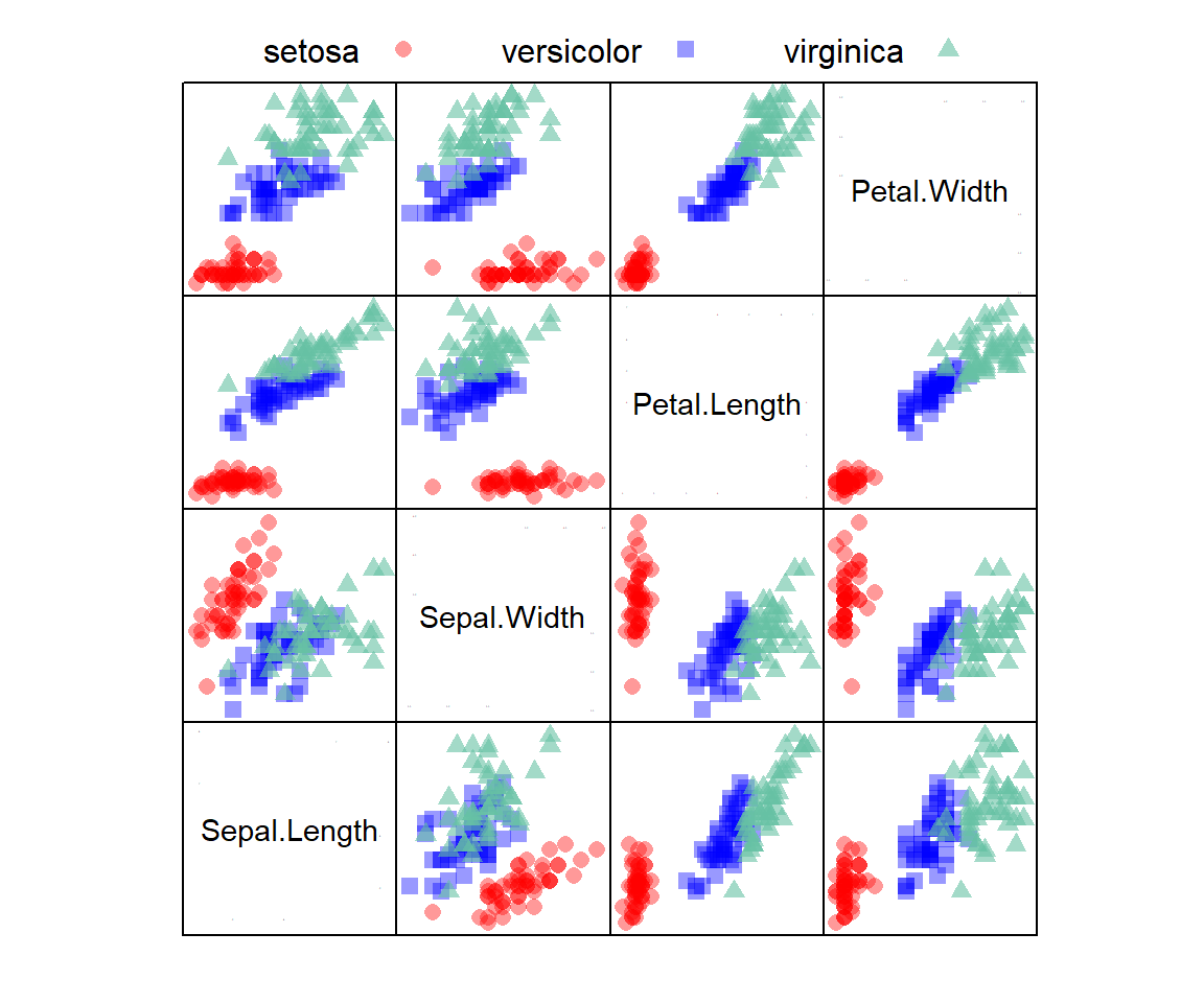
FIGURE 12.9: A scatterplot matrix showing associations of variables from the iris dataframe with species designations overlaid. Panels on the diagonal denote axes. For example, in the top-left plot the vertical and horizontal axes are Petal.Width and Sepal.Length, respectively.
Assume that we wish to create a predictive classification model for the iris species, using the iris dataset for training (70% of data) and testing (30% of data).
# Set a seed for reproducibility
set.seed(3)

# Create a data partition
trainID <- createDataPartition(iris$Species,
                                  p = 0.7,
                               list = FALSE)

trainData <- iris[trainID,] #70% training
testData <- iris[-trainID,] #30% testing
Here we employ a \(k\) nearest neighbor classifier (Hastie et al. 2009), which is based on the \(k\) closest samples to each individual sample in the training dataset199. The caret package currently allows a large number of other modelling approaches.
# Define training control with 10-fold cross-validation
ctrl <- trainControl(method = "cv", number = 10)

knn_model <- train(Species ~ ., # use all predictors
                   data = trainData,
                   method = "knn",
                   trControl = ctrl,
                   preProcess = c("center", "scale"),
                   tuneLength = 10
                  )
The caret::trainControl() function (Line 1 above) controls computational characteristics of the caret::train() function
Here method = "cv", number = 10 indicates the training control will use a resampling method with 10-fold cross-validation. This settings are initiated in train() using the trControl argument (Line 6). The training model itself is stipulated in Lines 3-8.
- The first argument,
Species ~ ., indicates that species designations should be considered a function of all the measured phenotypic variables (all columns other thanSpecies) in theirisdataframe (Line 3), - Line 5 asserts that the \(k\) nearest neighbor algorithm should be used as the clssifier.
- The code
preProcess = c("center", "scale")indicates that the mean should be subtracted from outcomes in corresponding columns, and these differences should be divided by the column standard deviation (see Example 8.5). - The code
tuneLength = 10gives the number of levels for each tuning parameter (in this case, the number of nearest neighbors, \(k\)) considered by the model.
We can evaluate the predictive effectiveness of the model with the “reserved” testData.
predictions <- predict(knn_model, testData)Below are the resulting user and producer accuracies, the \(\hat{\kappa}\) (kappa) statistic (a more conservative measure of classification effectiveness than the proportion of correctly classified items), and the confusion matrix (which counts correct designations on the diagonal).
asbio::Kappa(predictions, iris$Species[-trainID])$ttl_agreement
[1] 91.111
$user_accuracy
setosa versicolor virginica
100.0 93.3 80.0
$producer_accuracy
setosa versicolor virginica
100.0 82.4 92.3
$khat
[1] 86.7
$table
reference
class1 setosa versicolor virginica
setosa 15 0 0
versicolor 0 14 3
virginica 0 1 12\(\blacksquare\)
Exercises
-
With respect to operating systems, processors, and memory:
- Compare x86 and ARM processor architectures.
- Identify the the CPU processor architecture and operating system of your computer using R (see Example 12.1).
- Find the number of core processors on your machine using system shells (see Example 12.2)
- Find the amount of RAM on your computer using system shells (see Example 12.3).
-
Define the following terms:
- Motherboard
- Central processing unit (CPU)
- Random access memory (RAM)
- Primary memory
- Secondary memory
- Volatile memory
- Non-volatile memory
How many bits are in 5 gigabytes? How many are in 6 gibibytes?
-
What is the value of \(\beta\) in Eq (12.1) for binary and decimal systems?
-
With respect to precision…
- Write the decimal number 225.20 and 225.2 in scientific notation.
- What is the numeric precision 225.20 and 225.2?
-
With respect to binary expressions…
- Obtain the five bit binary sequence for the numbers 21 and 0.35, by hand. Check your answer using
dec2bin(). - Find the decimal number corresponding to the five bit binary sequences
11111,0.1101and10.10by hand by applying Eq (12.1). Check your answer usingbin2dec(). - Find the binary two’s complement expression for the decimal number -21.2 by hand. Check your answer using
dec2bin.twos(). - Using Eq. (12.1), find the decimal number corresponding to the two’s complement binary number
110.10. Check your answer usingbin2dec(). - Find the 64 bit binary expression for the decimal number \(-2\) (minus 2) using the function
bit64(), as shown in Example 12.15. Back-transform this binary representation to the decimal number by hand using Eq. (12.2). Use R functions likestrsplit()unlist(), etc.
- Obtain the five bit binary sequence for the numbers 21 and 0.35, by hand. Check your answer using
-
With respect to double precision…
- What is the level of for decimal fractional components in R, and all software that uses binary64 (see Section 12.7)? Why?
- What are the (non-infinite) minimum and maximum double precision values allowed by R. Why?
- What are the minimum and maximum integer values allowed by R? Why?
-
With respect to hexadecimal expressions…
- What does
310 =112 =316 mean? - What is the decimal representation of the hexadecimal code
B0? Why? (Hint: see Examples 12.17 and 12.18) - What is the hexadecimal code for the Unicode character
<? Why? - How would we code for the Unicode character
<in R?
- What does
-
With respect to internet and web topics…
- What is the internet protocol suite?
- Distinguish an IP address, a URL, and a domain name.
- Obtain your private IP address(es) using
ipconfig(cmd) orip addr(BASH).
Distinguish serial and parallel computing.