9 R Interfaces

“You should try things; R won’t break.”

- Duncan Murdoch, from R-help (May 2016)

9.1 Introduction

R can be interfaced with a non-native software package or language using a binding procedure, also called an application programming interface (API)⁹⁴. The binding provides glue code that allows R to work directly with foreign systems that extend its capacities. This can be done in two basic ways.

First, R-bindings for external, self-contained software programs can be used. This allows R-users to: 1) parameterize and initiate an external program using wrapper functions, and, 2) access the output from that program for further analysis and distillation. If one is using existing APIs, then these operations will generally not require knowledge of non-R languages (as the heavy lifting is being done with utility functions within particular R packages). One will, however, have to install the R package containing the API(s), and the software that one wishes to interface.

Second, one can harness useful characteristics of non-R languages by: 1) writing or utilizing source code for procedures in those languages, and 2) using APIs to run those processes in R, possibly following their compilation into entities called executable files (Section 9.1.3).

Although bindings for external software are considered briefly (Section 9.1.1), this chapter focuses primarily on interfaces of the second type, particularly linkages to the programming languages Fortran, C, C++, SQL, and Python. Brief backgrounds to those languages are provided here. These, however, should not be considered thorough introductions, given that: 1) I am not a computer language polyglot, and 2) my focus is to demonstrate how other languages can be interfaced with R, and not the languages themselves. Appropriate references to language resources are provided throughout the chapter⁹⁵.

To account for the frequent use of distinct computer languages in this chapter, the following chunk coloring conventions will be used hereafter in this book⁹⁶:

# R code

! Fortan code

// C and C++ code

# Python code

-- SQL code

:: Windows Command shell

9.1.1 R Bindings for Existing External Software

Many applications exist for interfacing R with extant, biologically-relevant software. For example, the R package arcgisbinding⁹⁷ allows R-based geoprocessing within ArcGIS Pro and ArcGIS Enterprise.

Example 9.1 \(\text{}\)
Here I establish a connection to the ArcGIS software package on my computer from within R.

library(arcgisbinding)

arc.check_product()

product: ArcGIS Pro (13.4.0.55405)
license: Advanced
version: 1.0.1.311 

\(\blacksquare\)

The R package igraph (Csárdi et al. 2025) provides C-bindings for an extensive collection of graph-theoretic tools that can be applied in biological settings, e.g., Aho, Derryberry, et al. (2023). Wrappers for open-source bioinformatics software include the R package RCytoscape, from the Bioconductor repository, which allows cross-communication between the popular Java-driven software for molecular networks Cytoscape; the R package dartR.popgen which interfaces with C-based STRUCTURE software for investigating population genetic structure; and the R package strataG (currently only available on GitHub) which can interface with STRUCTURE, along with the bioinformatics apps: CLUMPP, MAFFT, GENEPOP, fastsimcoal, and PHASE.

R can also be accessed from popular commercial software packages. This capacity is particularly prevalent for commercial statistical software, including SAS, SPSS, and MINITAB.

9.1.2 Interfacing With Non-R Languages

Code from other languages can be interfaced to R at the command line prompt, and within R functions. For instance, we have already considered the use of Perl regex calls for managing character strings in Ch 4 (Section 4.3), and the R Markdown document processing workflow is largely a chain of Markup language conversions (Section 2.10.2.1). Other examples include code interfaces from C, Fortran, C++, SQL, and Python (all formally considered in this chapter), MATLAB (via package R.matlab, Bengtsson (2022)), and Java (via package rJava, Urbanek (2021))⁹⁸.

9.1.2.1 Costs/Benefits of Interfacing Non-R Scripts

There are costs and benefits to creating/using interface scripts. Costs include:

• Scripts written in non-interpreted languages (e.g., C, Fortran, C++, see Section 9.1.3) will require compilation. Therefore it may be wise to limit such code to package-development applications (Ch 10) because R built-in procedures can facilitate this process during package building.
• Interfacing with older, low level languages (e.g., Fortran and C (Section 9.2)) increases the possibility for programming errors, often with serious consequences, including memory faults. That is, bugs bite (Chambers 2008)!
• Interfacing with some languages may increase the possibility for programs being limited to specific platforms.
• R programs can often be written more succinctly. For instance, Morandat et al. (2012) found that R programs are about 40% smaller than analogous programs written in C.

Despite these issues, there are a number of strong potential benefits. These include:

• A huge number of useful, well-tested, algorithms have been written in other languages, and it is often straightforward to interface these procedures with R.
• The system speed of other languages may be much better than R for many tasks. For instance, looping algorithms written in non-interpreted languages, are often much faster than corresponding procedures written in R.
• Non-OOP languages may be more efficient than R with respect to memory usage.

9.1.3 Interpreted and Compiled Languages

Along with many other useful languages (e.g., Python, JavaScript), R is generally run as an interpreted language. Interpreted code must be translated into binary before it can be executed. This process can slow down process run times, particularly if the process includes iterative procedures like loops. Non-interpreted (compiled) languages include C, Fortran, and Java. For those languages, a compiler (a translation program) is used to transform the source code into a target “object” language, which is generally binary (Ch 11). The end product of the compilation is called an executable file (Figure 9.1). Executables from other languages can be called from within R to run independently or to enhance R functions and procedures.

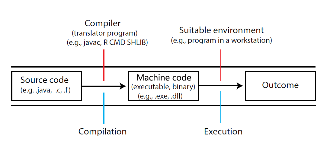
Figure 9.1: Creating an executable file in a compiled language.

9.1.4 Windows Shells

Compiling executables in Windows will require installation/access to appropriate compiler programs. These, in turn, may require initiation from a shell command line.

The Windows OS (as of Windows 10) has two built-in command line shells: the Command shell (also know as cmd.exe or cmd), which dates back to 1993, and PowerShell, which was introduced in 2006. For simplicity, I use the former shell here⁹⁹. The Command shell (and PowerShell) commands and processes for Windows differ in many respects from the POSIX (Portable Operating System Interface) compliant shells generally used by Unix-like systems. For instance, BASH¹⁰⁰ –the default shell for most UNIX-alike operating systems– is both a command-line interpreter and a highly flexible programming language. The BASH system is briefly considered in Ch 12, in the context of high performance computing (see Section 12.8.1).

Table 9.1 shows some Windows Command shell commands. Additional guidance can be found at the learn.microsoft.com website.

Table 9.1: Windows Command shell commands.

Command	Description
cd	Prints name of directory or changes directory
cd <address>	Navigate to location in <address>
cd\	Returns to the root dirctory
cd..	Navigate “up” one directory level
cls	Clears command line
dir	Lists files in directory
findstr	Search for a text string in a file (or multiple files)
<command> \? or help <command>	Returns help (if available) for <command>
systeminfo	Shows PC System Details
drivequery	Lists all installed drivers
ipconfig	Shows information about IP addresses and connections
tasklist	Prints current tasklist

Example 9.2 \(\text{}\)
The default home directory for my computer is: C:\Users\ahoken. To navigate to the root (parent) directory of this hierarchy, I could type cd/ (Table 9.1) in the Windows Command shell.

C:\Users\ahoken>cd/
C:\>

Note that the shell has the same command line prompt as R: >.

\(\blacksquare\)

Example 9.3 \(\text{}\)
What if I wanted to list all the R-Markdown files (those with an .rmd file extension) in the home directory for this book? I could navigate to the correct directory, and type dir /b *.rmd in the Windows Command shell:

C:\>cd C:\Users\ahoken\Documents\GitHub\Amalgam
C:\Users\ahoken\Documents\GitHub\Amalgam>dir /b *.rmd
01-Ch1.Rmd
02-Ch2.Rmd
03-Ch3.Rmd
04-Ch4.Rmd
05-Ch5.Rmd
06-Ch6.Rmd
07-Ch7.Rmd
08-Ch8.Rmd
09-Ch9.Rmd
10-Ch10.Rmd
11-Ch11.Rmd
12-Ch12.Rmd
13-references.Rmd
index.Rmd

The \b option in dir means: “use a bare format (no heading information or summary).” The asterisk, *, is a wildcard, indicating that only files with a .rmd extension should be listed.

To search for the text: "An Amalgam of R" in the R Markdown document index.rmd, I could use the findstr command:

C:\Users\ahoken\Documents\GitHub\Amalgam>findstr "\"An\ Amalgam\ of\ R\"" index.rmd
title: "An Amalgam of R"

Note that I escape both quotes and spaces in the string. The entire line of text containing the string is: title: "An Amalgam of R" and is part of the YAML header in index.rmd (Section 2.10.2.1). Note that some compatability with regular expressions is provided by findstr (Section 4.3.6). For more information type findstr \? in the Windows Command shell (Table 9.1).

\(\blacksquare\)

CAUTION!

The Windows Command shell is a powerful tool, and serious damage can be done to your computer through its misapplication. This is particularity true when running destructive commands, e.g., del, rmdir, format as an Administrator.

9.1.5 Interfacing with R Markdown/RStudio

Language and program interfacing with R can be greatly facilitated through the use of R Markdown chunks. This is because many languages other than R are supported by R Markdown, via knitr. The language definition for a particular R Markdown chunk is given by the first term in that chunk. For instance, ```{r } ``` initiates a conventional R code chunk, whereas ```{python }``` initiates a Python code chunk. Here are the current R Markdown language engines (note that items 52-64 are not explicit computer languages).

names(knitr::knit_engines$get())

 [1] "awk"         "bash"        "coffee"      "gawk"        "groovy"     
 [6] "haskell"     "lein"        "mysql"       "node"        "octave"     
[11] "perl"        "php"         "psql"        "Rscript"     "ruby"       
[16] "sas"         "scala"       "sed"         "sh"          "stata"      
[21] "zsh"         "asis"        "asy"         "block"       "block2"     
[26] "bslib"       "c"           "cat"         "cc"          "comment"    
[31] "css"         "ditaa"       "dot"         "embed"       "eviews"     
[36] "exec"        "fortran"     "fortran95"   "go"          "highlight"  
[41] "js"          "julia"       "python"      "R"           "Rcpp"       
[46] "sass"        "scss"        "sql"         "stan"        "targets"    
[51] "tikz"        "verbatim"    "theorem"     "lemma"       "corollary"  
[56] "proposition" "conjecture"  "definition"  "example"     "exercise"   
[61] "hypothesis"  "proof"       "remark"      "solution"    "glue"       
[66] "glue_sql"    "gluesql"    

As evident in the output above, R Markdown engines extend to compiled languages including Fortran (engine = fortran), C (engine = c) and C++, via the Rcpp package (engine = Rcpp).

9.1.6 Compilation for R Interfacing

Windows executable files compiled from source code will generally have an .exe or .cmd extension, whereas Mac OS executable files generally have have .app extension. For use in R, however, these files must be shared library executables, with .dll and .so extensions for Windows and Unix-alike (e.g., Mac-OS) operating systems, respectively¹⁰¹. Shared library objects are different from conventional executables in that they cannot be evaluated directly. In this case, R will be required as the executable entry point.

R provides shared library compilers for Fortran and C and several other languages via its SHLIB procedure, which is accessed from the Rcmd executable. The Rcmd program is located in the R bin directory, following a conventional download from CRAN, along with several other important R executables, including R.exe and Rgui.exe. Rcmd procedures are typically invoked from a shell (e.g., cmd.exe) using the format: R CMD procedure args. Here procedure is currently one of INSTALL, REMOVE, SHLIB, BATCH, build, check, Rprof, Rdconfig, Rdiff, Rd2pdf, Stangle, Sweave, config, open, and texify, and args defines arguments specific to the Rcmd command¹⁰². For example, the shell script:

R CMD SHLIB foo

would prompt the building of a shared library object from the user-defined script foo, which could be comprised, for example, of Fortran, C, or C++ source code¹⁰³. There are actually many ways to compile shared libraries for use in R.

• First, as noted above, one could compile a shared library from some script, foo, by running R CMD SHLIB foo at a shell command line. The shared library could then be loaded and called, using an appropriate foreign function interface. I apply this approach from the Windows Command shell in Example 9.5.
• Second, one could rely only on R Markdown engines (see Section 2.7 in Xie, Dervieux, and Riederer (2020)). In particular, one could write a script for a compiled language within a chunk with an approriate language engine. The chunk would be automatically compiled using SHLIB when running the chunk. The resulting shared library could then be loaded and called in a subsequent R chunk, using an appropriate foreign function interface, e.g., .Call() (see Section 9.2). Unfortunately, this process may be hampered by a number of factors, including non-administrator permissions and environmental path definitions, particularly on Windows computers.
• Third, one could use the inline facilitator package inline which compiles code using SHLIB, and creates an R function that calls a shared library, all from the R console (see Section 9.3.2).
• Finally, one could use a non-SHLIB compiler. For example, the GNU Compiler Collection (GCC) contained in Rtools. Rtools is a Windows toolchain, intended primarily for building packages (and R) from source code. Because R packages may include C, C++, and Fortran scripts, Rtools contains compilers for those languages¹⁰⁴. This method is used throughout Section 9.3.
  

9.2 Fortran and C

S, the progenitor of R, was created at a time when Fortran¹⁰⁵ routines dominated numerical programming, and R arose when C¹⁰⁶ was approaching its peak in popularity. As a result, strong connections to those languages, particularly C, remain in R¹⁰⁷. R contains specific base functions for interfacing with both C and Fortran executables: .C() and .Fortran() .

Recall that an R object of class numeric will be automatically assigned to base type double, although it can be coerced to base type integer (with information loss through the elimination of its “decimal” component).

as.integer(2.5)

[1] 2

Many other languages, however, do not automatically assign base types. Instead, explicit user-assignments for underlying base types are required.

If one is interfacing R with Fortran or C, only a limited number of base types are possible (Table 9.2), and one will need to use appropriate coercion functions for R objects if one wishes to use those objects in Fortran or C scripts¹⁰⁸. Interfaced C script arguments must be pointers and arguments in Fortran scripts must be arrays for the types given in Table 9.2.

Table 9.2: Correpsonding types for R, C, and Fortran. Table adapted from Chambers (2008).

R base type	R coercion function	C type	Fortran type
logical	as.integer()	int *	integer
integer	as.integer()	int *	integer
double	as.double()	double *	double precision
complex	as.complex()	Rcomplex *	double complex
charater	as.character()	char **	character*255
raw	as.character()	char *	none

Raw Fortran source code is generally saved as an .f, or (.f90 or .f95; modern Fortran) file, whereas C source code is saved as an .c file. One can create a file with the correct file type extension by using file.create().

Example 9.4 \(\text{}\)
For example, below I create a file called foo.f90 that I can open (from my working directory) in a text editor (e.g., Notepad) or IDE (e.g., RStudio) to build a Fortran script.

file.create("foo.f90")

\(\blacksquare\)

RStudio provides an IDE for C, allowing straightforward generation of .c files.

9.2.1 Compiling and Executing C and Fortran Programs

Notably, the SHLIB compilers will only work for Fortran code written as a subroutine¹⁰⁹ and C code written in void formats¹¹⁰. As a result, neither code type will return a value directly.

Example 9.5 \(\text{}\)
Here is a simple example for calling Fortran and C compiled executables from R to speed up looping. The content follows class notes created by Charles Geyer at the University of Minnesota. Clearly, the example could also be run without looping. Equation (9.1) shows the simple formula for converting temperature measurements in degrees Fahrenheit to degrees Celsius.

\[\begin{equation} C = 5/9(F - 32) \tag{9.1} \end{equation}\]

where \(C\) and \(F\) denote temperatures in Celsius and Fahrenheit, respectively.

Here is a Fortan subroutine for calculating Celsius temperatures from a dataset of Fahrenheit measures, using a loop.

subroutine FtoC(n, x)
integer n
double precision x(n)
integer i
do 100 i = 1, n
x(i) = (x(i)-32)*(5./9.)
100 continue
end

The Fortran code above consists of the following steps:

• On Line 1 a subroutine is invoked using the Fortran function subroutine. The subroutine is named FtoC, and has arguments x (the Fahrenheit temperatures) and n (the number of temperatures)
• On Line 2 the entry given for n is defined to be an integer (Table 9.2).
• On Line 3 we define x to be a double precision numeric vector of length n.
• On Line 4 we define that the looping index to be used, i, will be an integer.
• On Lines 5-7 we proceed with a Fortran do loop. The code do 100 i = 1, n means that the loop will 1) run initially up to 100 times, 2) has a lower limit of 1, and 3) has an upper limit of n. The code: x(i) = (x(i)-32)*(5./9.) calculates Eq. (9.1). The code 5./9. is used because the result of the division can be a non-integer. The code 100 continue allows the loop to continue to n.
• On Line 8 the subroutine ends. All Fortran scripts must end with end.

I save the code under the filename FtoC.f90, and transfer it to an appropriate directory (I use C:/Users/ahoken/Documents/Amalgam/Amalgam_Bookdown/scripts/). I then open a Windows shell editor.

I compile FtoC.f90 using the script R CMD SHLIB FtoC.f90. Thus, at the Windows Command shell I enter:

cd C:\Program Files\R\R-4.4.2\R\bin\x64  
R CMD SHLIB C:/Users/ahoken/Documents/Amalgam/Amalgam_Bookdown/scripts/FtoC.f90

Note the change from back slashes to (Unix-style) forward slashes when specifying addresses for SHLIB. The command above creates the compiled Fortran executable FtoC.dll. Specifically, the Fortran compiler, GNU Fortran (GCC), is used to create a Unix-style shared library FtoC.o. This file is then converted to a .dll file, aided by the RTools GCC 10/MinGW-w64 compiler toolchain. By default, the .dll is saved in the directory that contained the source code. Steps in the compilation process can be followed (with difficulty) in the cryptic shell output below:

Here is an analogous C loop function for converting Fahrenheit to Celsius.

void ftocc(int *nin, double *x)
{
  int n = nin[0];
  int i;
  for (i=0; i<n; i++)
    x[i] = (x[i] - 32) * 5 / 9;
}

The C code above consists of the following steps.

• Line 1 is a line break.
• On Line 2 a void function is initialized with two arguments. The code int *nin means “access the value that nin points to and define it as an integer.” The code double *x means: “access the value that x points to and define it as double precision.”
• Lines 8-9 define the C for loop. These loops have the general format: for ( init; condition; increment ) {statement(s); }. The init step is executed first and only once. Next the condition is evaluated. If true, the loop is executed. The syntax i++ literally means: i = i + 1. Note that code lines are ended with a semicolon, : and that indices (e.g., i) start at 0.

Once again, I save the source code, FtoCc.c, within an appropriate directory. I compile the code using the command R CMD SHLIB FtoCc.c. Thus, at the at the Windows Command shell I enter:

cd C:\Program Files\R\R-4.4.2\R\bin\x64  
R CMD SHLIB C:/Users/ahoken/Documents/Amalgam/Amalgam_Bookdown/scripts/FtoCc.c 

This creates the shared library executable FtoCc.dll.

Below is an R-wrapper that can call the Fortran executable, call = "Fortran", the C executable, call = "C", or use R looping, call = "R". Several new functions are used. On Line 10 the function dyn.load() is used to load the shared Fortran library file FtoC.dll, while on Lines 14-15 dyn.load() loads the shared C library file FtoCc.dll. Note that the variable nin is pointed toward n, and x is included as an argument in dyn.load() on Line 15. On Line 11 the function .Fortran() is used to execute FtoC.dll, and on Line 16 .C() is used to execute FtoCc.dll.

F2C <- function(x, call = "R"){
  n <- length(x)
  if(call == "R"){
    out <- 1:n
    for(i in 1:n){
    out[i] <- (x[i] - 32) * (5/9)
    }
  }
  if(call == "Fortran"){
    dyn.load("C:/Users/ahoken/Documents/Amalgam/Amalgam_Bookdown/scripts/FtoC.dll")
    out <- .Fortran("ftoc", n = as.integer(n), x = as.double(x))
  }
  if(call == "C"){
    dyn.load("C:/Users/ahoken/Documents/Amalgam/Amalgam_Bookdown/scripts/FtoCc.dll",
             nin = n, x)
    out <- .C("ftocc", n = as.integer(n), x = as.double(x))
  }
  out
}

Here I create \(10^8\) potential Fahrenheit temperatures that will be converted to Celsius using (unnecessary) looping.

x <- runif(100000000, 0, 100)
head(x)

[1] 76.391 68.578 12.061 71.886 66.711 72.958

Note first that the Fortran, C, and R loops provide identical temperature transformations. Here are first 6 transformations:

head(F2C(x[1:10], "Fortran")$x)

[1]  24.661  20.321 -11.077  22.159  19.284  22.755

head(F2C(x[1:10], "C")$x)

[1]  24.661  20.321 -11.077  22.159  19.284  22.755

head(F2C(x[1:10], "R"))

[1]  24.661  20.321 -11.077  22.159  19.284  22.755

However, the run times are dramatically different¹¹¹. The C executable is much faster than R, and the venerable Fortran executable is even faster than C!

system.time(F2C(x, "Fortran"))

   user  system elapsed 
   0.64    0.14    0.78 

system.time(F2C(x, "C"))

   user  system elapsed 
   0.55    0.33    0.89 

system.time(F2C(x, "R"))

   user  system elapsed 
   5.59    0.33    5.95 

\(\blacksquare\)

9.3 C++

C++ (pronounced see plus plus) is a high-level, general-purpose, programming language that is well known for its simplicity, efficiency, and flexibility¹¹². C++ was originally intended to be an extension of C. Although its scope now greatly exceeds this intent, C++ syntax remains very similar to C. For instance, like C:

• C++ is a compiled language.
• Lines of C++ code end with semicolons, ;.
• C++ comment annotations begin with \\.
• The for loop syntax for C++ is: for (init; condition; increment).
• c++ index values start at 0, meaning that the last index value will be n - 1.
• Square braces, [], can be used for subsetting. Although, see content regarding Rcpp C++ types below.
• c++ Logical operators are similar to those used in R. For example, == is the Boolean equals operator, ! is the unary operator for not, and the operators for and and or are && and ||, respectively.
• C++ Boolean designations,true and false are used (instead of TRUE and FALSE, like R).

The major difference between C and C++ is that C++ supports objects and object classes, whereas C does not. Helpful online C++ tutorials and references can be found at https://www.learncpp.com/ and https://en.cppreference.com/w/cpp, respectively. As advanced resources, Wickham (2019) recommends the books: Effective C++ (Meyers 2005) and Effective STL (Meyers 2001)¹¹³.

9.3.1 Rcpp

The R package Rcpp (Eddelbuettel 2013; Eddelbuettel and Balamuta 2018; Eddelbuettel et al. 2023) provides a stand-in for the R API, with a consistent set of C++ classes (Eddelbuettel and François 2023). As a result, the package allows users to employ the many useful characteristics of C++ –including fast loops, efficient calls to functions, and access to advanced data structures, including ordered maps¹¹⁴ and double-ended queues¹¹⁵, while enjoying the benefits of R –including straightforward manipulation of vectors and matrices. As Wickham (2019) notes:

“I do not recommend using C for writing new high-performance code. Instead write C++ with Rcpp. The Rcpp API protects you from many of the historical idiosyncracies of the R API, takes care of memory management for you, and provides many useful helper methods.”

Useful resources for Rcpp include extensive vignettes from the package itself, Chapter 25 from Wickham (2019), and the online document Rcpp for everyone (Tsuda 2020).

In order to use Rcpp, users will require additional toolchains, including a dedicated C++ compiler.

• Windows users will need Rtools. Use of Rtools will require that its installation be along an defined environmental path.
• Mac-OS users will require the Xcode command line tools.
• Linux users can use: `sudo apt-get install r-base-dev`.

Example 9.6 \(\text{}\)
As a first step, Eddelbuettel and Balamuta (2018) recommend running a minimal example to ensure that the Rcpp toolchain is working. For instance:

library(Rcpp)

evalCpp("2 + 2")

[1] 4

Here the function Rcpp::evalCpp() creates a compiled C++ shared library, specified in evalCpp(), from the text string "2 + 2". This step is accomplished via the function Rcpp::cppFunction() (see Example 9.8 below). The evalCpp() function then calls shared library, using .Call(), to obtain a result in R.

\(\blacksquare\)

9.3.1.1 Data Types

Recall from Section 2.3.6 that R base types correspond to a C typedef alias called an SEXP (S-expression). Rcpp provides dedicated C++ classes for most of the 24 SEXP types. Some of these are shown in Table 9.3.

Table 9.3: Correpsonding types for R, C++, and Rcpp. Table adapted from Tsuda (2020).

R type	C++ (scalar)	Rcpp (scalar)	Rcpp::Vecor	Rcpp::Matrix
logical	bool	-	LogicalVector	LogicalMatrix
integer	int	-	IntegerVector	IntegerMatrix
numeric	double	-	NumericVector	NumericMatrix
complex	complex	Rcomplex	ComplexVector	ComplexMatrix
character	char	String	CharacterVector	CharacterMatrix
Date	-	Date	DateVector	-
POSIXct	time_t	Datetime	DatetimeVector	-

Rcpp also has types for R base types list and S4, and R class dataframe. These are called using Rcpp::List, Rcpp::S4, and Rcpp::Dataframe, respectively.

Rcpp objects of type Vector, Matrix, Dataframe and List can be created by first specifying their class names.

Example 9.7 \(\text{}\)
The code (not run) below creates Rcpp::Vector objects called v. Corresponding R code is commented above C++ code.

// v <- rep(0, 3)
NumericVector v (3);

// v <- rep(1, 3)
NumericVector v (3,1);

// v <- c(1,2,3) 
// [[Rcpp::plugins("cpp11")]]
NumericVector v = {1,2,3}; 

// v <- 1:3
IntegerVector v = {1,3};

// v <- as.logical(c(1,1,0,0))
LogicalVector v = {1,1,0,0};

// v <- c("a","b")
CharacterVector v = {"a","b"};

Note that curly braces {} are used to initialize the NumericVector object on Line 9, and the IntegerVector, LogicalVector, and CharacterVector objects on Lines 12, 15, 18, respectively. This reflects C++ 11 grammar¹¹⁶. C++11 can be enabled with the comment: // [[Rcpp::plugins("cpp11")]] (Line 8).

Here I create Rcpp::Matrix objects named m:

// m <- matrix(0, nrow=2, ncol=2)
NumericMatrix m(2);

// m <- matrix(v, nrow=2, ncol=3)
NumericMatrix m( 2, 3, v.begin());

The matrix object on Line 4 above is filled using a Vector object named v. This is facilitated with the Rcpp Vector member function begin() (Section 9.3.1.2).

Below is a Rcpp::Dataframe with columns comprised of Vectors named v1 and v2.

// df <- data.frame(v1, v2)
DataFrame df = DataFrame::create(v1, v2);

Here is a Rcpp::List containing Vectors v1 and v2.

// L <- list(v1, v2)
List L = List::create(v1, v2);

\(\blacksquare\)

9.3.1.2 Member Functions

Rcpp has useful C++ member functions (functions that can be used to interact with data of specific user-defined types) for its Vector, Matrix, List and Dataframe types. Specifically, for a member function foo that corresponds to a type defined for an object bar, I would run foo on bar by typing bar.foo(). Note that Rcpp member functions in Table 9.4 with generic names, e.g., length() are analogous to R methods for particular S3 and S4 classes (Section 8.6).

Table 9.4: Some C++ member functions for Rcpp types. To run a member function mfunc() on an appropriate object x, I would type: x.mfunc().

Function	Vector	Matrix	Dataframe	List	Operation
length(), size()	X		X	X	Returns length of List or Vector, or number of Dataframe columns
names()	X		X	X	Names attribute
sort()	X			X	Sorts object into ascending order
get_NA()	X			X	Returns NA values
is_NA(x)	X			X	Returns true if a vector element specified by x is NA
nrows()		X	X		Retruns number of rows
ncols()		X	X		Retruns number of columns
begin()	X		X	X	Returns iterator pointing to first element
end()	X		X	X	Returns iterator pointing to end of object
fill_diag(x)		X			Fill Matrix diagonal with scalar x

9.3.1.3 C++ Math With R-like Functions

Rcpp contains R-like functions that extend C++ scalar mathematical functions, which woould otherwise be applied via the <cmath> header file. These allow users to capitalize on the vectorized efficiencies of R, within C++ scripts, while using R-like grammar (Table 9.5).

Table 9.5: C++ <math.h> functions for a scalar, s, and R-like Rcpp functions for a Vector, v.

C++ scalar, s	Rcpp Vector, v	Operation
log2(s)		\(\log_2\) of s.
log(s)	log(v)	natural log(s) of s or elements in v.
log10(s)	log10(v)	\(\log_{10}\) of s or elements in v.
exp(s)	exp(v)	\(\exp()\) of s or elements in v.
abs(s)	abs(v)	absolute value(s) of s or elements in v.
abs(s, n)	pow(v,n)	raises s or elements in v to nth power.
round(s,d)	round(v,d)	rounds s or elements in v to d digits.
sin(s)	sin(v)	sine of s or elements in v.
cos(s)	cos(v)	cosine of s or elements in v.
tan(s)	tan(v)	tangent of s or elements in v.
asin(s)	asin(v)	arcsine of s or elements in v.
acos(s)	acos(v)	arccosine of s or elements in v.
atan(s)	atan(v)	arctangent of s or elements in v.
	min(v)	minimum value of v
	max(v)	maximum value of v
	sum(v)	sum of v
	cumsum(v)	cumulative sum of v
	cumprod(v)	cumulative product of v
	range(v)	min and max of v
	mean(v)	mean of v
	median(v)	median of v.
	sd(v)	standard deviation of v
	var(v)	variance of v.
	na_omit(v)	returns Vector with NA elements in v deleted
	is_na(v)	labels NA elements in v TRUE
	sapply(v,fun)	applies C++ function fun to vector v
	lapply(v,fun)	applies C++ function fun to vector v; returns List
	cbind(x1, x2,...)	combines Vector or Matrix in x1, x2

9.3.1.4 Inline C++ Code

The function Rcpp::cppFunction() allows users to specify C++ code for a single function as a character string at the R command line (see minimal Example 9.6 above). The function compiles C++ code, and creates a link to the resulting shared library. It then defines an R function that uses .Call() to invoke the library.

Example 9.8 \(\text{}\)
Here is a simple function for generating numbers from a Fibonacci sequence. See Question 6 in the Exercises from Ch 8.

cppFunction(
    'int fibonacci(const int x) {
        if (x == 0) return(0);
        if (x == 1) return(1);
        return (fibonacci(x - 1)) + fibonacci(x - 2);
    }')

• On Line 2, the C++ function name finbonacci is defined. The function output and the class of the argument x are both defined to be int (integers).
• On Lines 3-4 the first two numbers in the sequence are defined based on Boolean operators.
• On Line 5, later numbers in the sequence (\(n > 2\)) are defined.

The result from the script is an R function that loads the compiled shared library, based on the C++ function fibonacci, using .Call().

fibonacci

function (x) 
.Call(<pointer: 0x00007ffd80cc1820>, x)

Here we use the R function to generate the 10th Fibonacci number.

fibonacci(10)

[1] 55

\(\blacksquare\)

The R function Rcpp::sourceCpp()allows general compilation of C++ scripts that may contain multiple functions.

9.3.1.5 Formal C++ Scripts

We can use Rcpp to facilitate the creation of more conventional C++ scripts (not just character strings of C++ code). These will have the general form (Tsuda 2020):

#include <Rcpp.h>
using namespace Rcpp;

// [[Rcpp::export]]
RETURN_TYPE FUNCTION_NAME(ARGUMENT_TYPE ARGUMENT){
  //function contents 
  return RETURN VALUE;
}

• On Line 1, the code #include <Rcpp.h> loads the Rcpp header file Rcpp.h. In several C-alike languages (C, C++, C-obj), header files can be use to provide definitions for functions, variables, and (in the case of C++) new class definitions (Table 9.3). See Chapter 6 in R Core Team (2024c).
• The (optional) code using namespace Rcpp (Line 2) allows direct access to Rcpp classes and functions. Without this designation, an Rcpp function or class foo would require the call Rcpp::foo, instead of simply, foo.
• The comment: // [[Rcpp::export]]： (Line 4) serves as a compiler attribute, and demarks the beginning of C++ code that will be accessible from R. The Rcpp::export attribute is required (by Rcpp) for any C++ script to be run from R. The attribute currently requires specification as a comment, because it will be unrecognized within most compilers.
  
• For RETURN_TYPE FUNCTION_NAME(ARGUMENT_TYPE ARGUMENT){ (Line 5) users must specify data types of functions, a function name, argument types, and arguments.
• return RETURN VALUE; is required if function output is desired.

As before, this process compiles the C++ code into shared library, and creates an R function (with the same name as the C++ function) that calls the shared library (Example 9.8). In R Markdown, one can check and debug this process by calling R to run this function from within the chunk containing the associated C++ script, by using the subsequent code form:

/*** R
FUNCTION_NAME
*/

where FUNCTION_NAME is the name of the resultant R function.

Example 9.9 \(\text{}\)
RStudio provides an IDE for C++ scripts. Further, a C++ file obtained using File>New File>C++ contains an example Rcpp-formatted C++ example function, named timesTwo, that multiplies some number by two:

#include <Rcpp.h>
using namespace Rcpp;

// [[Rcpp::export]]
NumericVector timesTwo(NumericVector x) {
  return x * 2;
}

Note use of the Rcpp type NumericVector to define function output and values for the argument, x (Line 5).

Running the code above compiles timesTwo into a shared library, and creates an R function (with the same name) in the global environment. This function loads the shared library for use in R.

timesTwo(5)

[1] 10

\(\blacksquare\)

Example 9.10 \(\text{}\)
As a series of biological examples, we will create C++ functions (using Rcpp tools) for measuring the diversity of ecological communities. Below is a function for calculating relative abundances of species in a community (individual species abundance divided by the sum of species abundances).

#include <Rcpp.h>
using namespace Rcpp;

// [[Rcpp::export]]
NumericVector relAbund(NumericVector x) {
  int n = x.length();
  double total = 0;
  for(int i = 0; i < n; ++i) {
    total += x[i];
  }
  NumericVector rel = x/total;
  return rel;
}

The function relAbund is a mixture of standard C++ code and calls to C++ classes and procedures from Rcpp. In particular,

• On Lines 1 and 2, I bring in the Rcpp.h header file, and load the Rcpp namespace.
• On Line 4, I include the comment, // [[Rcpp::export]] to prompt R to recognize code below the line.
• On Line 6, I specify the data types of the function output, NumericVector, the function name, the data type for the argument NumericVector, and the argument itself, x.
• Lines 7-8 are preliminary steps for the loop codified on Lines 9-11. On Line 7, an integer object n is created by find the number of observation in x. This is done with the Rcpp Vector member function length() (Table 9.4) with the call x.length().
  
• Lines 9-11 comprise a standard C/C++ looping approach for calculating total abundance (the sum of x). The useful operator += adds the right operand to the left operand and assign the result to the left operand.
• On Lines 12-13 relative abundance are calculated and the resulting NumericVector is returned.

Recall (Example 6.17) that the dataset vegan::varespec describes the abundance of vascular plants, mosses, and lichen species for sites in a Scandinavian taiga/tundra ecosystem. Here I run the function for the site represented in row 1 (site 18).

library(vegan)
data(varespec)

relAbund(as.vector(varespec[1,], "double"))

 [1] 0.00616592 0.12477578 0.00000000 0.00000000 0.19955157 0.00078475
 [7] 0.00000000 0.00000000 0.01793722 0.02320628 0.00000000 0.01816143
[13] 0.00000000 0.00000000 0.05235426 0.00022422 0.00145740 0.00000000
[19] 0.00145740 0.00134529 0.00000000 0.24360987 0.24069507 0.03923767
[25] 0.00336323 0.00201794 0.00257848 0.00280269 0.00280269 0.00257848
[31] 0.00000000 0.00000000 0.00089686 0.00022422 0.00022422 0.00000000
[37] 0.00134529 0.00022422 0.00695067 0.00022422 0.00000000 0.00000000
[43] 0.00280269 0.00000000

I ensure that the C++ shared library relAbund views varespec[,1] as double precision by specifying mode = "double" in as.vector().

Recall (Example 8.20) that species relative abundances are used in calculating measures of \(\alpha\)-diversity. The code below calculates Simpson diversity (Eq. (8.2)) from a vector of abundance data.

#include <Rcpp.h>
#include <cmath>
using namespace Rcpp;

// [[Rcpp::export]]
double simpson(NumericVector x) {
  NumericVector y = na_omit(x);
  double total = sum(y); 
  NumericVector relsq = pow(y/total, 2);
  return 1 - sum(relsq);
}

Note that on Line 7, I have dramatically simplified the calculation of relative abundance by replacing the for loop in relAbund with the R-like Vector function Rcpp::sum() (Table 9.5). Other R-like C++ functions used above include na_omit() (Line 6) Rcpp::pow() and (Line 8). The former allows handling data with missing values.

simpson(as.vector(varespec[1,], mode = "double"))

[1] 0.82171

\(\blacksquare\)

Example 9.11 \(\text{}\)
The code below shows how one would run some simple mathematical operation in C++ (see Table 9.5) that combine C++ scripting at the R command line with formal C++ grammar, including header files.

src <- 
'
#include <Rcpp.h> 
#include <math.h>

using namespace Rcpp;
// [[Rcpp::export]]

List math_demo(){
  double a = sin(3);
  double b = log(3);
  double c = log2(3);
  NumericVector v = {1,2,3};
  double d = min(v);
  NumericVector e = log(v);
  return List::create(Named("a") = a,
                      Named("b") = b,
                      Named("c") = c,
                      Named("d") = d,
                      Named("e") = e);
}'

sourceCpp(code = src)
math_demo()

$a
[1] 0.14112

$b
[1] 1.0986

$c
[1] 1.585

$d
[1] 1

$e
[1] 0.00000 0.69315 1.09861

\(\blacksquare\)

9.3.1.6 Accessing/Manipulating Data Types Components

Rcpp data type objects can generally be subset using (), [], or member functions. Both () and [] can be used with Rccp::NumericVector, Rcpp::IntegerVector and CharacterVector types. Rcpp::Dataframe objects require [], whereas Rcpp::Matrix, require () for subsetting.

Example 9.12 \(\text{}\)
Here is a long-winded C++ function that demonstrates Rcpp subsetting using Rcpp::NumericVector objects, an Rcpp::NumericMatrix object, and an Rcpp::Dataframe object.

#include <Rcpp.h>
using namespace Rcpp;
// [[Rcpp::export]]
List subsets(){
  // Create Vectors
  NumericVector nv = {10, 20, 30, 40, 50, 60};
  nv.names() = CharacterVector({"A","B","C","D","E","F"});
  NumericVector nv2 = nv + 1;
  NumericVector nv3 = nv + nv2; // Rcpp allow elementwise Vector operations
  // Create Matrix
  NumericMatrix nm(2, 3, nv.begin());
  // Create Dataframe
  DataFrame df = DataFrame::create(Named("V2") = nv2, Named("V3") = nv3);
  // Indexes
  NumericVector id1 = {1,3};
  CharacterVector id2 = {"A","D","E"};
  LogicalVector id3 = {false, true, true, true, false, true};
  // Vector subsets based on indexes
  int x1 = nv[0]; 
  int x2 = nv["C"]; 
  NumericVector x3 = nv[id1];
  NumericVector x4 = nv[id2];
  NumericVector x5 = nv[id3];
  // Matrix subsets
  double x6 = nm(0 , 1); // Row 0 (first row) and column 1 (2nd column)
  NumericVector x7 = nm(1 , _ );  // Row 1 (2nd row)
  NumericVector x8 = nm( _ , 0);  // Column 0 (1st column)
  NumericVector x9 = nm.column(0);  // Column 0 (1st column)
  //Dataframe subsets
  NumericVector x10 = df[0];
  NumericVector x11 = df["V3"];
    
return List::create(Named("Result1") = x1, Named("Result2") = x2, 
                    Named("Result3") = x3, Named("Result4") = x4, 
                    Named("Result5") = x5, Named("Result6") = x6,
                    Named("Result7") = x7, Named("Result8") = x8, 
                    Named("Result9") = x9, Named("Result10") = x10,
                    Named("Result11") = x11);
}

subsets()

$Result1
[1] 10

$Result2
[1] 30

$Result3
 B  D 
20 40 

$Result4
 A  D  E 
10 40 50 

$Result5
 B  C  D  F 
20 30 40 60 

$Result6
[1] 30

$Result7
[1] 20 40 60

$Result8
[1] 10 20

$Result9
[1] 10 20

$Result10
[1] 11 21 31 41 51 61

$Result11
[1]  21  41  61  81 101 121

• As before, I call the Rcpp.h header file, apply the Rcpp namespace, and designate // [[Rcpp::export]] (Lines 1-3).
• On Line 4, C++ function is defined to have List output. No arguments are defined because the goal is to demonstrate Rcpp data type subsetting and manipulation, using only objects created within the function.
• On Lines 6-9, I create three NumericVector objects. The latter two are on elementwise transformations facilitated by Rcpp sugar operators.
• On Line 11, I create a NumericMatrix filled with elements from the Vector nv, using the Matrix deque member function begin(). Note that Rcpp matrices are built by column, given a vector input.
• On Line 13, I create a two column Dataframe comprised of the Vector objects nv2 and nv3. using the Matrix deque member function begin().
• On Line 15-17, three Vector objects that will be used for subsequent subsetting are created.
• On Lines 19-23, the objects x1, x2, x3, x4 and x5 are created by subsetting the Vector, nv.
• On Lines 25-28, the objects x6, x7, x8, and x9 are created by subsetting the Matrix, nm.
• On Lines 30-31, the objects x10 and x11 are created by subsetting the Dataframe, df.
• On Lines 33-38, the subset objects are assembled into a List and are returned by the function.

\(\blacksquare\)

Example 9.13 \(\text{}\)
We now know enough to extend our scalar function for Simpson’s diversity (Example 9.10) to a function that can handle matrices –the conventional format for biological community datasets.

#include <Rcpp.h>
using namespace Rcpp;
// [[Rcpp::export]]
NumericVector simpson(NumericMatrix x) {
  CharacterVector rn = rownames(x);
  NumericVector out = x.nrow();
  out.names() = rn;
  int n = out.size();
    
    for(int i = 0; i < n; ++i) {
    NumericVector temp = na_omit(x(i , _ ));
    double total = sum(temp); 
    NumericVector relsq = pow(temp/total, 2);
    out[i] = 1 - sum(relsq);
    }
 
  return out;
}

• As in previous examples, I first call the Rcpp.h header file, apply the Rcpp namespace, and define the // [[Rcpp::export]] compiler attribute (Lines 1-3).
• The function output will be a NumericVector (of Simpson’s diversities of sites) and will require a NumericMatrix for its argument x, with sites in rows and species in columns (Line 4).
• Lines 5-8 generate objects (out and n) that will be used in a subsequent loop.
• Lines 10-15 define a loop that populates out with Simpson’s diversities. The code: NumericVector temp = na_omit(x(i , _ )); creates a NumericVector object, temp, consisting of non-missing values in the \(i\)th row of x.
  
• ON Line 17 out is returned.

Here we apply our function to the entire vegan::varespec dataset.

simpson(as.matrix(varespec))

     18      15      24      27      23      19      22      16      28 
0.82171 0.76276 0.78101 0.74414 0.84108 0.81819 0.80310 0.82477 0.55996 
     13      14      20      25       7       5       6       3       4 
0.81828 0.82994 0.84615 0.83991 0.70115 0.56149 0.73888 0.64181 0.78261 
      2       9      12      10      11      21 
0.55011 0.49614 0.67568 0.50261 0.80463 0.85896 

We see that our C++ function is much faster than the widely-used function vegan::diversity(), which relies on an R for loop.

m <- matrix(nrow = 10^6, ncol = 10, data = rnorm(10^7) + 10)
system.time(simpson(m))

   user  system elapsed 
   0.30    0.05    0.34 

system.time(vegan::diversity(m, "simpson"))

   user  system elapsed 
   3.04    0.11    3.16 

\(\blacksquare\)

9.3.2 The inline package

The inline R package (Sklyar, Eddelbuettel, and Francois 2025) extends the capacities of Rcpp::evalCpp(), Rcpp::cppFunction() and Rcpp::sourceCpp() by allowing users to create, compile, and run functions written in any language supported by R CMD SHLIB, including C, Fortran, C++, and C-obj, from the R command line.

Example 9.14 \(\text{}\)
Consider the following example –based on ? inline::cfunction()– of a simple C function that raises every value in a numeric vector to the third power.

library(inline)

code.cube <- "
      int i;
      for (i = 0; i < *n; i++)
        x[i] = x[i]*x[i]*x[i];
"
cube.fn <- cfunction(signature(n="integer", x="numeric"), code.cube,
                     language = "C", convention = ".C")

cube.fn(20, 1:20)

$n
[1] 20

$x
 [1]    1    8   27   64  125  216  343  512  729 1000 1331 1728 2197 2744
[15] 3375 4096 4913 5832 6859 8000

Note that code.cube, is a character string containing C-script (Lines 3-7). The script on Lines 9 and 10 calls inline::cfunction() to compile the string into a C shared library executable using SHILB. The shared library will be called automatically using .C(), allowing cube.fn used as an R function on Line 9. The object cube.fn has an unusual combination of characteristics. It is a function of base type closure:

typeof(cube.fn)

[1] "closure"

However, it is also S4,

isS4(cube.fn)

[1] TRUE

with the following slots:

slotNames(cube.fn)

[1] ".Data" "code" 

The code slot can be obtained using the function inline::code()

code(cube.fn)

  1: #include <R.h>
  2: 
  3: 
  4: void file8c068f83924 ( int * n, double * x ) {
  5: 
  6:       int i;
  7:       for (i = 0; i < *n; i++)
  8:         x[i] = x[i]*x[i]*x[i];
  9: 
 10: }

Note that the text string has been converted to a C void function, as required by SHLIB. The header call #include <R.h> provides a built-in R API for C code.

The .Data slot contains R code that is run by interpreter when cube.fn() is called. Note that the function uses .Primitive() to call the appropriate shared library under a temporary pointer name.

cube.fn@.Data

function (n, x) 
.Primitive(".C")(<pointer: 0x00007ffdef4f1380>, n = as.integer(n), 
    x = as.double(x))
<environment: 0x00000193e1d06fd8>

\(\blacksquare\)

9.4 SQL and Databases

Biological databases have grown exponentially in size and number (Sima et al. 2019). Because of this trend, biological databases are often housed in web-accessible warehouses including the National Center for Biotechnology Information (NCBI), dataBase for Gene Expression Evolution (Bgee), and the European life-sciences infrastructure for biological information (ELIXIR).

Databases are often assembled in a Database Management System (DBMS) format. A DBMS will contain one or more rectangular row/column storage units called tables. Rows in tables are called records and columns are called fields or attributes.

Many DBMS formats have evolved based on the Structured Query Language (SQL). Although SQL is an American National Standards Institute (ANSI) and International Organization for Standardization (ISO) standard, there are many variants of SQL, and software for managing these languages is often proprietary (e.g., Oracle, Microsoft SQL Server) and potentially expensive. Despite this variety, SQL dialects generally use the same basic SQL commands (Table 9.6), and processes. For example, as a general rule, SQL table fields can be accessed with a period operator. That is, a column, bar, in table foo is specified as foo.bar. SQL guidance can be found at a large number of websites, including the developer site W³.

Table 9.6: Important SQL commands. Out of convention, SQL commands here are shown in upper-case. SQL keywords, however, are not case sensitive. That is, select is the same as SELECT.

Command	Meaning
SELECT	Extracts data from a database
FROM	Used with SELECT. A clause identifying a database
UPDATE	Updates data in a database
DELETE	Deletes data from a database
CREATE TABLE	Creates a new table
WHERE	Filters records from a table
AND	Filters records based on more than one condition
OR	Filters records based on more than one condition
BETWEEN	Selects values within a given range

9.4.1 DBI

The R package DBI (R Special Interest Group on Databases (R-SIG-DB), Wickham, and Müller 2024; James 2009) currently allows communication with 30 SQL-driven DBMS formats. Each supported DBI DBMS uses its own R package. For instance, the SQLite DBMS is interfaced with the package RSQLite (which will be installed with DBI), and the MySQL DBMS can be interfaced using the package RMySQL. The RMariaDB package can be used to interface either MySQL or the DBMS MariaDB. Opening a DBMS connection will constrain users to the SQL nuances of the selected DBMS. We will concentrate on the non-proprietary DBMS SQLite here.

library(DBI)

library(RSQLite)

Example 9.15 \(\text{}\)
As a simple first example, we will create a database using “internal” R dataframes. First we establish a SQLite DBMS connection using dbConnect().

con <- dbConnect(SQLite(), ":memory:")
con

<SQLiteConnection>
  Path: :memory:
  Extensions: TRUE

Unlike many other DBMS frameworks that may require a username, password, host, port, and other information, SQLite only requires a path to the database¹¹⁷. The argument ":memory:" specifies a special path that results in an “in-memory” database.

Notably, the con database is an S4 object:

isS4(con)

[1] TRUE

Here we append the asbio::world.emission dataframe to the database using dbWriteTable().

library(asbio)
data(world.emissions)
dbWriteTable(con, "emissions", world.emissions)

We see that the table (renamed emissions) now exists in the database.

dbListTables(con)

[1] "emissions"

Below we use SQL script (within the R function DBI::dbSendQuery()) to access information from the database table emissions. In particular –using the commands SELECT, FROM, WHERE, AND, and BETWEEN– I query the columns coal_co2 and gas_co2, with respect to the United States, for the years 2016 to 2019.

us <- dbSendQuery(con, "SELECT coal_co2, gas_co2 
                  FROM emissions 
                  WHERE country = 'United States' 
                  AND year BETWEEN 2016 AND 2019")

To access all columns from emissions, I could have used the SQL command: "SELECT * FROM emissions.

Here I fetch the query result using dbFetch():

us.fetch <- dbFetch(us)
us.fetch

  coal_co2 gas_co2
1   1378.2  1509.0
2   1337.5  1491.8
3   1282.1  1653.0
4   1094.7  1706.9

The fetched result is a dataframe.

class(us.fetch)

[1] "data.frame"

One should clear queries using DBI::dbClearResult(). This will free all computational resources (local and remote) associated with a query result.

dbClearResult(us)

Databases can contain multiple tables. Here I append the asbio::C.isotope dataframe to the database:

data(C.isotope)
dbWriteTable(con, "isotopes", C.isotope)

There are now two tables in the database (although they are not relational).

dbListTables(con)

[1] "emissions" "isotopes" 

When finished accessing a DBMS, one should always close the DBMS connection.

dbDisconnect(con)

\(\blacksquare\)

In R Markdown one can use the SQL of the chosen DBMS directly, by specifying ```{sql, connection = con}``` when initiating code chunks, where con is the name of the database connection (see Section 9.1.5). This approach is often required for complex operations.

Example 9.16 \(\text{}\)
Reconsidering Example 9.15 we have:

con <- dbConnect(SQLite(), ":memory:")
dbWriteTable(con, "emissions", world.emissions)

Here I directly specify an SQL query (in SQL).

SELECT coal_co2, gas_co2
FROM emissions
WHERE country = 'United States'
AND year BETWEEN 2016 AND 2019;

coal_co2	gas_co2
1378.2	1509.0
1337.5	1491.8
1282.1	1653.0
1094.7	1706.9

Reflecting the requirements of several DBMS variants, I end SQL the statements above with a semicolon, ;.

dbDisconnect(con)

\(\blacksquare\)

9.4.2 Relational DBMS

Thus far, the justification for an interfaced DBMS may seem vague, since similar data management results could be obtained by subsetting R lists.

The advantages of creating a DBMS become clearer when considering a relational DBMS (RDBMS). An RDBMS allows the straightforward linking of multiple database tables via a common value identifier stored in the tables (Fig 9.2).

Figure 9.2: A relational database from the gene expression database Bgee. Several tables are linked via the identifier SpeciesID. Figure taken from Sima et al. (2019).

Example 9.17 \(\text{}\)
In this example we will impart relational characteristics to a database based on two R dataframes, asbio::Rabino_CO2 and asbio::Rabino_del13C, obtained from (Rubino et al. 2013). The datasets record CO\(_2\) and \(\delta^{13}\)C levels from Law Dome and South Pole, Antarctica for a 1000 year timespan. Exact effective date records, precision, and measurement depths all vary for the entries (see Example 7.5), prompting the creation of two separate datasets.

First, I create mean effective date records to eventually provide a single-entry label field for each dataset, based on the effective.age of samples.

data(Rabino_CO2)
data(Rabino_del13C)

library(tidyverse)
AvgCO2df <- Rabino_CO2 |>
  group_by(effective.age) |>
  summarise(AvgDdepth = mean(depth), 
            AvgCO2 = mean(CO2), 
            AvgUncertainty = mean(uncertainty))

Avg13Cdf <- Rabino_del13C |>
  group_by(effective.age) |>
  summarise(AvgDepth = mean(depth), 
            Avgd13C = mean(d13C.CO2), 
            AvgUncertainty = mean(uncertainty))

names(Avg13Cdf)[1] <- names(AvgCO2df)[1] <- "EffectiveAge"
AvgCO2df$EffectiveAge <- as.integer(unlist(AvgCO2df[,1]))
Avg13Cdf$EffectiveAge <- as.integer(unlist(Avg13Cdf[,1]))

The resulting summary dataframes, AvgCO2df and AvgC13df, do not contain measures from the same effective dates. Specifically, 114 (out of 189) AvgCO2df effective age records do not occur in AvgC13df.

length(AvgCO2df$EffectiveAge) - 
  length(which(AvgCO2df$EffectiveAge %in% Avg13Cdf$EffectiveAge))

[1] 114

And 10 (out of 85) AvgC13df effective age records do not occur in AvgCO2df.

length(Avg13Cdf$EffectiveAge) - 
  length(which(Avg13Cdf$EffectiveAge %in% AvgCO2df$EffectiveAge))

[1] 10

Nonetheless, we can easily join the datasets in a DBMS, and use their effective ages, to simultaneously query them.

We first request a SQLite database connection.

con <- dbConnect(SQLite(), ":memory:")

We then add AvgCO2df and AvgC13df to the database as tables.

dbWriteTable(con, "CO2", AvgCO2df)
dbWriteTable(con, "d13C", Avg13Cdf)

There are several database joins we can specify using SQL, including LEFT JOIN and RIGHT_JOIN. Assume that we have two tables in a database , A and B.

If I request A LEFT JOIN B, then the result set will include:

• Records in A and B with corresponding labels.
• Records (if any) in A without corresponding labels in B. In this case, B entries are given NULL values.

Conversely, if I request A RIGHT JOIN B, then the result set will include:

• Records in B and A with corresponding labels.
• Records (if any) in B without corresponding labels in A. In this case, A entries are given NULL values.

SELECT AvgCO2, d13C.Avgd13C, CO2.EffectiveAge
FROM CO2 LEFT JOIN d13C
ON d13C.EffectiveAge = CO2.EffectiveAge
WHERE CO2.EffectiveAge > 1990;

AvgCO2	Avgd13C	EffectiveAge
352.22	-7.8410	1991
353.73	-7.8820	1992
353.94	-7.8883	1993
357.11	NA	1994
359.65	NA	1996
361.78	-8.0600	1998
368.02	-8.0695	2001

In the SQL code above, I specify a LEFT JOIN.

• On Line 1, I specify the fields whose data I want to consider jointly, AvgCO2, d13C.Avgd13C, and the reference field I wish to use, CO2.EffectiveAge, i.e., the EffectiveAge field in the CO2 table.
• On Line 2, I specify the join: CO2 LEFT JOIN d13C.
• On Line 3, I identify the fields used to join the tables.
• On Line 4, I limit the printed results to CO2.EffectiveAge values greater than 1990.

Note that in the output above there are two effective ages, 1994 and 1996, with CO\(_2\) records but no \(\delta^{13}\)C records.

SELECT AvgCO2, d13C.Avgd13C, CO2.EffectiveAge
FROM CO2 RIGHT JOIN d13C
ON d13C.EffectiveAge = CO2.EffectiveAge
WHERE CO2.EffectiveAge > 1990;

AvgCO2	Avgd13C	EffectiveAge
352.22	-7.8410	1991
353.73	-7.8820	1992
353.94	-7.8883	1993
361.78	-8.0600	1998
368.02	-8.0695	2001

The RIGHT JOIN SQL statement above is identical to the previous statement except for the Line 2 command: CO2 RIGHT JOIN d13C. In the output, complete \(\delta^{13}\)C records for the requested effective age range are returned (note that ages 1994 and 1996 are omitted). While not required by the query, corresponding records for CO\(_2\) also exist, and are reported.

dbDisconnect(con)

\(\blacksquare\)

9.4.3 Creating an SQLite database

Thus far we have used package dataframes to populate an SQLite database connection. A more realistic application would be assembling an SQLite database from related but intentionally separated data files.

Example 9.18 \(\text{}\)

\(\blacksquare\)

9.5 Python

Python, whose image logo is shown in Fig 9.3, is similar to R in several respects. Python was formally introduced in the early 90s, is an open source OOP language that is rapidly gaining popularity, and its user code is evaluated in an on-the-fly manner. That is Python, like R, is an interpreted language.

Figure 9.3: The symbol for Python, a high-level, general-purpose, programming language.

Like R, comments in Python are made using the metacharacter #¹¹⁸. Boolean operators are similar, although, while the unary operator for “not” in R is !, in Python it actually is not, and Python uses True and False instead of TRUE and FALSE.

There are, however, several fundamental differences between Python and R. These include the fact that while white spaces in R code (including tabs) simply reflect coding style preferences –for example, to increase code clarity– Python indentations denote code blocks¹¹⁹. That is, Python indentations serve the same purpose as R curly braces. Another important difference is that R object names can contain a . (dot), whereas in Python . means: “attribute in a namespace.” That is, in Python . serves the same role as $ in R list and dataframe objects (Section 3.1.4). Recall that the . operator is used in a similar way in SQL language queries of database tables (Section 9.4). Useful guidance for converting R code to analogous Python code can be found here.

Python can be downloaded for free from (https://www.python.org/downloads/), and can be activated from the Windows command line using the command py, and activated from the Mac and Unix/Linux command line using the command python. General guidance for the Python language can be found at (https://docs.python.org/) and many other sources including these books.

C:\>py
Python 3.11.3 (tags/v3.11.3:f3909b8, Apr  4 2023, 23:49:59) [MSC v.1934 64 bit (AMD64)] on win32
Type "help", "copyright", "credits" or "license" for more information.
>>>

Note that the standard command line prompt for the Python shell is >>>. We can exit Python from the command line by typing quit().

9.5.1 reticulate

Because our primary interest is interfacing Python and R, and not Python itself, we will use R as our base of operations. This will require the R package reticulate (Ushey, Allaire, and Tang 2023).

# install.packages("reticulate")
library(reticulate)

RStudio (via reticulate) can be used as an IDE for Python¹²⁰. In this capacity RStudio will:

• Generate a Python specific environment (to allow separate listing of Python and R objects).
• Call separate R and Python environments, depending on which language is currently used in a chunk. Python code can be run in R Markdown by defining python (instead of r) as the first option in an R Markdown chunk.

We can specify a path to the Python system (allowing us to use different versions of Python) with reticulate::use_python(). This is important because specific versions of Python may dramatically affect the usability of basic Python functions. The code below specifies use of the current version of Python, as accessed with Sys.which(), which finds full paths to program executables.

use_python(Sys.which("python"))

A Python command line interface can also be called directly in R using:

repl_python()

Python can be closed from the resulting interface (returning one to R) by typing:

exit

One can obtain information about the version of Python currently being used by reticulate by running the function retuclate::py_config (in R).

reticulate::py_config()

python:         C:/Users/ahoken/AppData/Local/Programs/Python/Python311/python.exe
libpython:      C:/Users/ahoken/AppData/Local/Programs/Python/Python311/python311.dll
pythonhome:     C:/Users/ahoken/AppData/Local/Programs/Python/Python311
version:        3.11.3 (tags/v3.11.3:f3909b8, Apr  4 2023, 23:49:59) [MSC v.1934 64 bit (AMD64)]
Architecture:   64bit
numpy:          C:/Users/ahoken/AppData/Local/Programs/Python/Python311/Lib/site-packages/numpy
numpy_version:  1.24.2

NOTE: Python version was forced by RETICULATE_PYTHON_FALLBACK

Example 9.19 \(\text{}\)

The following are Python operations, run directly from RStudio.

2 + 2

4

The Python assignment operator is =.

x = 2
x + x

4

Here we see the aforementioned importance of indentation.

if x < 0:
  print("negative")
else:
  print("positive")

positive

Lack of an indented “block” following if will produce an error. Indentations in code can be made flexibly (e.g., one space, two space, tab, etc.) but they should be used consistently.

\(\blacksquare\)

9.5.2 Packages

Like R, Python consists of a core language, a set of built-in functions, modules, and libraries (i.e., the Python standard library), and a vast collection (\(>200,000\)) of supplemental libraries. Imported libraries are extremely important in Python because its distributed version has limited functional capabilities (compared to R). A number of important Python supplemental libraries, each of which contain multiple packages, are shown in Table 9.7.

Table 9.7: Important Python supplemental libraries. For more information use hyperlinks.

Library	Purpose
sumpy	Fundamental package for scientific computing
scipy	Mathematical functions and routines
matplotlib	2- and 3-dimensional plots
pandas	Data manipulation and analysis
sympy	Symbolic mathematics
bokeh	Interactive data visualizations

We can install Python packages and libraries using the pip package manager for Python¹²¹. Installation only needs to occur once on a workstation (similar to install.packages() in R). Following installation, one can load a package for a particular work session using the Python function import (analogous to library() in R)¹²².

Installation of a Python package, foo, with reticulate, via pip, can be accomplished using the function reticulate::py_install (in R)¹²³.

py_install("foo", pip = TRUE)

Example 9.20 \(\text{}\)
For example, to install the scipy library I use the command:

py_install("scipy", pip = TRUE) # Run in R, if scipy has not been installed

To load the scipy library I could use the Python function import():

import scipy 

\(\blacksquare\)

9.5.3 Functions in Packages

Functions within Python packages are obtained using a package.function syntax. Here I import numpy and run the function pi (which is contained in numpy).

import numpy
numpy.pi

3.141592653589793

If we are writing a lot of numpy functions, Python will allow you to define a simplified library prefix. For instance, here I created a shortcut for numpy called np and use this shortcut to access the numpy functions pi() and sin().

import numpy as np
np.sin(20 * np.pi/180) # sin(20 degrees)

0.3420201433256687

Use of the command from numpy import * would cause names of functions from NumPy to overwrite functions with the same name from other packages. That is, we could run numpy.pi simply using pi.

Example 9.21 \(\text{}\)
Here we import the package pyplot from the library matplotlib, rename the package plt, and create a plot (Fig 9.4) using the function pyplot.plot() (as plt.plot()) by calling:

import matplotlib.pyplot as plt
plt.plot(range(10), 'bo')

Figure 9.4: Creating a Python plot using R.

In Line 2, the command range(10) creates a sequence of integers from zero to ten. This is used as the first argument of plt.plot(), which specifies the plot \(x\)-coordinates. If \(y\) coordinates are not specified in the second argument, \(x\)-coordinates will be reused as \(y\) coordinates. The command 'bo' places blue filled circles at \(x\),\(y\) coordinates. Documentation for matplotlib.pyplot.plot() can be found at the matplotlib.org website.

\(\blacksquare\)

9.5.4 Data Types

There are four major built-in dataset storage classes in Python: lists, tuples, sets, and dictionaries (Table 9.8).

Table 9.8: The four Python dataset storage types.

Storage type	Example	Entry characteristics
List	["hot","cold"]	Changeable, Duplicates OK
Tuple	("hot","cold")	Unchangeable, Duplicates OK
Set	{"hot","cold"}	Unchangeable, Duplicates not OK
Dictionary	{"temp":["hot", cold"]}	Changeable, Duplicates not OK

All four classes track element order and can be used to simultaneously storage different types of data, e.g., character string and numbers.

We can make a Python list, which can contain both text and numeric data, using square brackets or the function list().

a = [20, 7, "Hi", 7, "end"]

Classes of Python objects can be identified with the Python function type().

type(a)

<class 'list'>

An empty list can be specified as []

empty = []
empty

[]

Like R, we can index list elements using square brackets. Importantly, like C-alike languages, indices start at 0. That is, a[0] refers to the first element of the list a.

a[0]

20

And the third element would be:

a[2]

'Hi'

As with R, square brackets can also be used to reassign list values

a[3] = 10
a

[20, 7, 'Hi', 10, 'end']

We can use the function append() to append entries to the end of a list. For instance, to append the number 9 to the object a in the previous example, I would type:

a.append(9)
a

[20, 7, 'Hi', 10, 'end', 9]

The function appendleft() can be used to efficiently append entries to the beginning of an object of class deque (from the Python collections package). The function deque() can be used to convert a list into a deque (double ended queue).

from collections import deque

a = deque(a)
type(a)

<class 'collections.deque'>

a.appendleft(0)
a

deque([0, 20, 7, 'Hi', 10, 'end', 9])

Unlike a Python list, a data object called a tuple, which is delineated using parentheses, contains elements that cannot be changed:

b = (1,2,3,4,5)
b[0]

1

b[0] = 10 # produces error

Multidimensional numerical arrays, including matrices, can be created using functions from numpy. Here we define:

\[\boldsymbol{B} = \begin{bmatrix} 1 & 4 & 5 \\ 9 & 7.2 & 4 \end{bmatrix}\]

B = np.array([[1, 4, 5], [9, 7.2, 4]])
type(B)

<class 'numpy.ndarray'>

We see that B is an object of class numpy.ndarray (meaning numpy n-dimensional array).

B

array([[1. , 4. , 5. ],
       [9. , 7.2, 4. ]])

Mathematical matrix operations can be easily applied to numpy.ndarray objects. Here I find \(\boldsymbol{B} - 5\)

B - 5

array([[-4. , -1. ,  0. ],
       [ 4. ,  2.2, -1. ]])

Extensive linear algebra tools are contained in the libraries numpy and scipy.

9.5.5 Mathematical Operations

Basic Python mathematical operators are generally (but not always) identical to R. For instance, note that for exponentiation ** is used instead of ^ (Table 9.9). This convention is also used by several other programming languages, including Fortran.

Table 9.9: Basic Python mathematical functions and operators.

Operator	Operation	To find	We type
+	addition	\(2 + 2\)	2 + 2
-	subtraction	\(2 - 2\)	2 - 2
*	multiplication	\(2 \times 2\)	2 * 2
/	division	\(\frac{2}{3}\)	2/3
**	exponentiation	\(2^3\)	2**3
sqrt(x)	\(\sqrt{x}\)	\(\sqrt{2}\)	numpy.sqrt(2)
factorial(x)	\(x!\)	\(5!\)	numpy.math.factorial(5)
log	\(\log_e\)	\(\log_e(3)\)	numpy.log(3)
pi	\(\pi = 3.141593 \dots\)	\(\pi\)	numpy.pi
inf	\(\infty\)	\(\infty\)	float('inf')
-inf	\(-\infty\)	\(-\infty\)	float('-inf')

Symbolic derivative solutions to functions can be obtained using functions from the library sympy. Results from the package functions can be printed in LaTeX for pretty mathematics.

py_install("sympy", pip = TRUE) # run in R if sympy hasn't been installed

Example 9.22 \(\text{}\)
Here we solve: \[\frac{d}{dx} 3e^{-x^2}\]

from sympy import *
x = symbols ('x')
fx = 3 * exp(-x ** 2)
print(diff(fx))

\[- 6 x e^{- x^{2}}\]

In Line 2, x is defined symbolically using the sympy.symbols() function. The variable x is used as a term in the expression fx in Line 3. The function fx is differentiated in Line 4 using the function sympy.diff().

\(\blacksquare\)

Integration in Python can be handled with the function quad() in scipy.

Example 9.23 \(\text{}\)
Here we find: \[\int_0^1 3e^{-x^2} dx\]

To perform integration we must install the scipy.integrate library using pip and bring in the function quad().

from scipy.integrate import quad

We then define the integrand as a Python function using the function def(). That is, def() is analogous to function() in R.

def f(x):
  return 3 * np.exp(-x**2)

We now run quad() on the user function f with the defined bounds of integration.

quad(f, 0, 1)

(2.240472398437281, 2.487424042782217e-14)

The first number is the value of the definite integral (in this case, the area under the function f from 0 to 1). The second is a measure of the absolute error in the numerical approximation.

\(\blacksquare\)

9.5.6 Reading in Data

Data in delimited files, including .csv files, can be read into Python using the numpy function loadtxt().

Example 9.24 \(\text{}\)
Assume that we have a comma separated dataset, named ffall.csv, located in the Python working directory, describing the free fall properties of some object over six seconds, with columns for observation number, time (in seconds), altitude (in mm) and uncertainty (in mm). The Python working directory (which need not be the same as the R working directory in RStudio) can be identified using the function getcwd() from the library os.

import os
os.getcwd()

'C:\\Users\\ahoken\\Documents\\GitHub\\Amalgam'

We can load freefall.csv using:

obs, time, height, error = np.loadtxt("ffall.csv", 
delimiter = ",", skiprows = 1, unpack = True)

The first row was skipped (using skiprows = 1) because it contained column names and those were re-assigned when I brought in the data. Note that, unlike R, columns in the dataset are automatically attached to the global environment upon loading, and will overwrite objects with the same name.

height/1000 # height in meters

array([0.18 , 0.182, 0.178, 0.165, 0.16 , 0.148, 0.136, 0.12 , 0.099,
       0.083, 0.055, 0.035, 0.005])

File readers in pandas are less clunky (and more similar to R). We can bring in freefall.csv using the function pandas.read_csv():

py_install("pandas")  # Run if pandas is not installed 

import pandas as pd # run in a Python chunk
ffall = pd.read_csv('ffall.csv')
ffall

    obs  time  height  error
0     1   0.0     180   3.50
1     2   0.5     182   4.50
2     3   1.0     178   4.00
3     4   1.5     165   5.50
4     5   2.0     160   2.50
5     6   2.5     148   3.00
6     7   3.0     136   2.50
7     8   3.5     120   3.00
8     9   4.0      99   4.00
9    10   4.5      83   2.50
10   11   5.0      55   3.60
11   12   5.5      35   1.75
12   13   6.0       5   0.75

The object ffall is a Pandas DataFrame, which is different in several respects, from an R dataframe. Column arrays in ffall can be called using the syntax: ffall., or by using braces. For instance:

ffall.height

0     180
1     182
2     178
3     165
4     160
5     148
6     136
7     120
8      99
9      83
10     55
11     35
12      5
Name: height, dtype: int64

ffall["height"]

0     180
1     182
2     178
3     165
4     160
5     148
6     136
7     120
8      99
9      83
10     55
11     35
12      5
Name: height, dtype: int64

\(\blacksquare\)

In RStudio, R and Python (reticulate) sessions are considered separately. In this process, when accessing Python from R, R data types are automatically converted to their equivalent Python types. Conversely, When values are returned from Python to R they are converted back to R types. It is possible, however, to access each from the others’ session.

The reticulate operator py allows one to interact with a Python session directly from the R console. Here I convert the pandas DataFrame ffall into a recognizable R dataframe, within R.

ffallR <- py$ffall

Which allows me to examine it with R functions.

colMeans(ffallR)

     obs     time   height    error 
  7.0000   3.0000 118.9231   3.1615 

On Lines 1 and 2 in the chunk below, I bring in the Python library pandas into R with the function reticulate:import(). The code pd <- import("pandas", convert = FALSE) is the Python equivalent to: import pandas as pd.

pd <- import("pandas", convert = FALSE)

As expected, the column names constitute the names attribute of the dataframe ffallR.

names(ffallR)

[1] "obs"    "time"   "height" "error" 

The ffall dataset, however, has different characteristics as a Python object. Note that in the code below the pandas function read_csv() is accessed using pd$read_csv() instead of pd.read_csv() because an R chunk is being used.

ffallP <- pd$read_csv("ffall.csv")

The names attribute of the pandas DataFrame ffallP, as perceived by R, contains over 200 entities, many of which are provided by the built-in Python module statistics. Here are the first 20.

head(names(ffallP), 20)

 [1] "abs"        "add"        "add_prefix" "add_suffix" "agg"       
 [6] "aggregate"  "align"      "all"        "any"        "apply"     
[11] "applymap"   "asfreq"     "asof"       "assign"     "astype"    
[16] "at"         "at_time"    "attrs"      "axes"       "backfill"  

I can use these entities to obtain statistical summaries of each column array, revealing an approach for R/Python syntheses.

ffallP$mean()

obs         7.000000
time        3.000000
height    118.923077
error       3.161538
dtype: float64

ffallP$var()

obs         15.166667
time         3.791667
height    3495.243590
error        1.512147
dtype: float64

ffallP$kurt()

obs      -1.200000
time     -1.200000
height   -0.692166
error     0.445443
dtype: float64

For further analysis in R these expression will need to be explicitly converted to R objects using the function py_to_r().

trans <- ffallP$transpose() # transpose matrix
transR <- py_to_r(trans)

apply(transR, 1, mean)

     obs     time   height    error 
  7.0000   3.0000 118.9231   3.1615 

9.5.7 Python versus R

R generally allows much greater flexibility than Python for explicit statistical analyses and graphical summaries. For example, the Python statistics library Pymer4 actually uses generalized linear mixed effect model (see Aho (2014)) functions from the R package lme4 to complete computations. Additionally, Python tends to be less efficient than R for pseudo-random number generation¹²⁴, since it requires looping to generate multiple pseudo-random outcomes (see Van Rossum and Drake (2009)).

Example 9.25 \(\text{}\)
Here I generate \(10^8\) pseudo-random outcomes from a continuous uniform distribution (processor details footnoted in Example 9.5).
R:

system.time(ranR <- runif(1e8))

   user  system elapsed 
   2.54    0.09    2.64 

Python:

import time
import random
ranP = []

start_time = time.time()
for i in range(0,9999999):
  n = random.random()
  ranP.append(n)
time.time() - start_time

6.071754217147827

The operation takes much longer for Python than R.

The Python code above requires some explanation. On Lines 1 and 2, the Python modules time and random are loaded from the Python standard library, and on Line 3 an empty list ranP is created that will be filled as the loop commences. On Line 5, the start time for the operation is recorded using the function time() from the module time. On Line 6 a sequence of length \(10^8\) is defined as a reference for the index variable i as the for loop commences. On Lines 7 and 8 a random number is generated using the function random() from the module random and this number is appended to ranP. Note that Lines 7 and 8 are indented to indicate that they reside in the loop. Finally, on Line 9 the start time is subtracted from the end time to get the system time for the operation.

\(\blacksquare\)

On the other hand, the system time efficiency of Python may be better than R for many applications, including the management of large datasets (Morandat et al. 2012).

Example 9.26 \(\text{}\)
Here I add the randomly generated dataset to itself in R:

system.time(ranR + ranR)

   user  system elapsed 
   0.14    0.19    0.33 

and Python:

start_time = time.time()
diff = ranP + ranP
time.time() - start_time

0.20841383934020996

For this operation, Python is faster.

\(\blacksquare\)

Of course, IDEs like RStudio allow, through the package reticulate, simultaneous use of both R and Python systems, allowing one to draw on the strengths of each language.

Exercises

1. The Fortran script below calculates the circumference of the earth (in km) for a given latitude (measured in radians). For additional information, see Question 6 from the Exercises in Ch 2. Explain what is happening in each line of code below.

subroutine circumf(x, n)
double precision x(n)
integer n
x = cos(x)*40075.017
end

2. Create a file circumf.f90 containing the code and save it to an appropriate directory. Take a screen shot of the directory.

3. Compile circumf.f90 to create circumf.dll. In Windows this will require the shell script:

cd Root part of address\bin\x64  
R CMD SHLIB Appropriate directory/circumf.f90

      You will have to supply your own Root part of address, and Approriate directory will be the directory containing circumf.f90.
      Take a screenshot to show you have created circumf.dll. Running the shell code may require that you use the shell as an Administrator.)

4. Here is a wrapper¹²⁵ for circumf.dll. Again, you will have to supply Approriate directory. Explain what is happening on Lines 2, 4, and 5. And, finally, run: cearthf(0:90).

cearthf <- function(latdeg){
  x <- latdeg * pi/180
  n <- length(x)
  dyn.load("Appropriate directory/circumf.dll")
  out <- .Fortran("circumf", x = as.double(x), n = as.integer(n))
  out
}

5. Here is a C script that is identical in functionality to the Fortran script in Q. 1. The header #include <math.h> (see Section 9.3.2) allows access to C mathematical functions, including cos(). Describe what is happening on Lines 7-10.

#include <math.h>


void circumc(int *nin, double *x)
{
  int n = nin[0];
  int i;
  for (i=0; i<n; i++)
    x[i] = (cos(x[i]) * 40075.017);
}

6. Repeat Qs, 2 and 3 for the C subroutine circumc.

7. Here is an R wrapper for circumc.dll. Explain what is happening on Lines 4-6 and run: cearthc(0:90).

cearthc <- function(latdeg){
  x <- latdeg * pi/180
  n <- length(x)
  dyn.load("Appropriate directory/circumc.dll",
           nin = n, x)
  out <- .C("circumc", n = as.integer(n), x = as.double(x))
  out
}

8. Complete Problem 5 (a-f) from the Exercises in Ch 2 using C++ via Rcpp. The code below completes part (a) and (b). Note the use of decimals to enforce double precision.

library(Rcpp)

src <- 
'
#include <Rcpp.h> 
#include <math.h>

using namespace Rcpp;
// [[Rcpp::export]]

List Q8(){
  double a = 1 + 3./10. + 2;
  double b = (1. + 3.)/10. + 2;
  return List::create(Named("a") = a,
                      Named("b") = b);
}'

sourceCpp(code = src)
Q8()

$a
[1] 3.3

$b
[1] 2.4

9. Using Rcpp, Create a C++ function for calculating the Satterthwaite degrees of freedom (see Q 2 from the Exercises in Ch 8). Test using the data: x <- c(1,2,3,2,4,5) and y <- c(2,3,7,8,9,10,11).
10. Make a Python list with elements "pear", "banana", and "cherry". (a) Extract the second item in the list. (b) Replace the first item in the list with "melon". (c) Append the number 3 to the list. .
11. Make a Python tuple with elements "pear", "banana", and "cherry". (a) Extract the second item in the tuple. (b) Replace the first item in the tuple with "melon". Was there an issue? (c) Append the number 3 to the tuple. Was there an issue?
12. Using def(), write a Python function that will square any value x, and adds a constant c to the squared value of x.
13. Call Python from R to complete Problem 5 (a-h) from the Exercises in Ch 2. Document your work in R Markdown.