3 Data Objects, Packages, and Datasets
“In God we trust. All others [must] have data.”
- Edwin R. Fisher, cancer pathologist
3.1 Data Storage Objects
Depending on who you talk to62, there are five primary types of data storage objects in R. These are: (atomic) vectors, matrices, arrays, dataframes, and lists63.
3.1.1 Vectors
Historically (and confusingly), the concept of an R “vector” can be traced directly to the earliest object-class system defined in the S language64. From this inception, an R vector is either an atomic vector –thus belonging one of the six atomic vector types: logical, integer, numeric, complex, character and raw– or an object of either class expression or class list. Objects of class expression generally contain mathematical calls or symbols that can be evaluated with the function eval() (see Section 2.9.5). Objects of class list are formally considered in Section 3.1.5.
Recall that R classes were introduced in Section 2.3.7, and that several fundamental classes were listed in Table 2.1. Because of their importance, the first eight classes shown in Table 2.1 classify vector types, and the first six specifically classify atomic vectors.
3.1.1.1 Atomic vectors
Atomic vectors constitute “the essential bottom layer” of R data (Chambers 2008). This is evident when viewing the relationship of atomic vectors to other data storage objects (Fig 3.1).
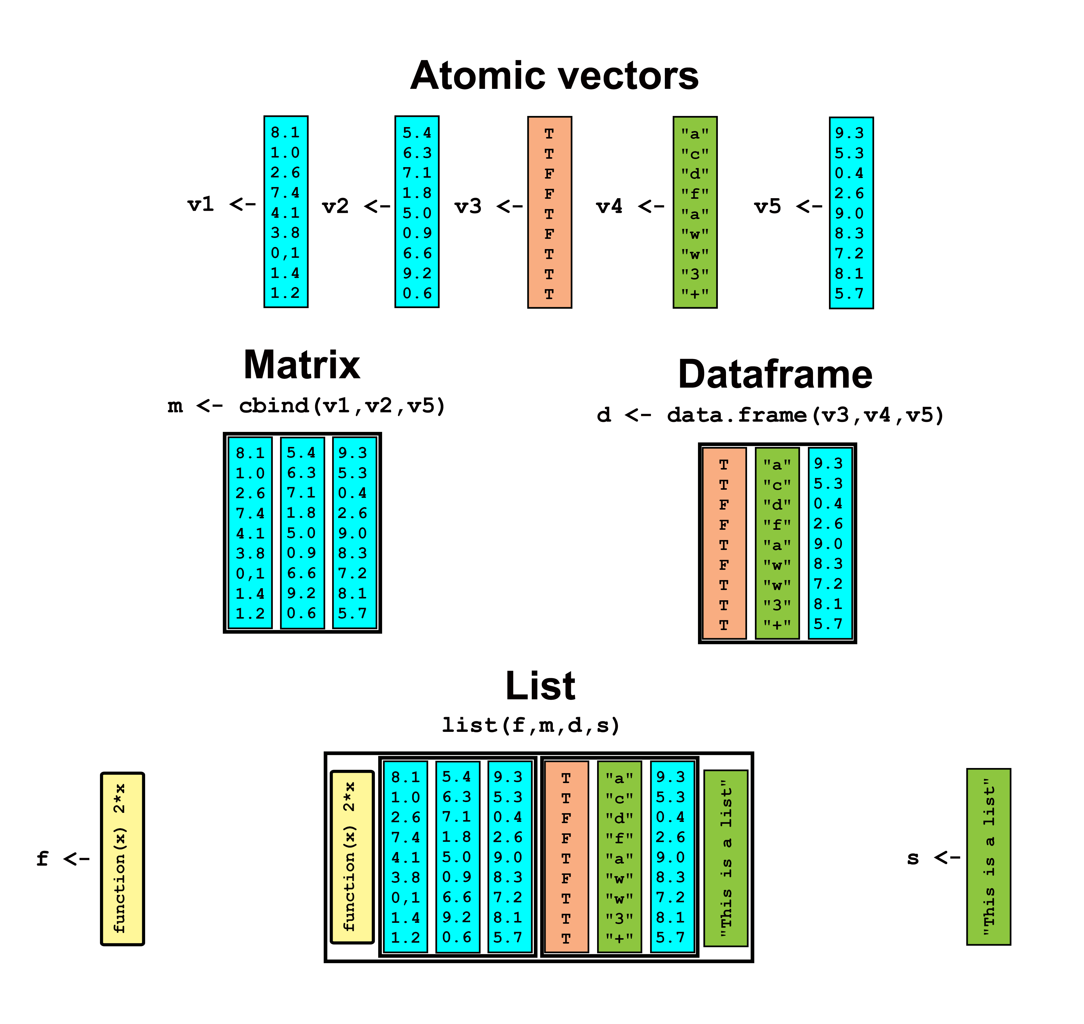
FIGURE 3.1: An example of R atomic vectors as building blocks for more complex data storage objects. Five atomic vectors are shown. Three are numeric (colored blue), one is logical (colored peach), and one is a character vector (light green). All atomic vectors can be assembled using c(). For example, v1 <- c(8.1, 1.0, 2.6,...). The numeric vectors are incorporated into a single matrix (which can have only one data storage mode), using cbind(). One of the numeric vectors, along with the character and logical vectors are incorporated into a dataframe (which can have multiple data storage modes). Finally, the matrix and dataframe are brought into a list, along with an anomolous function and character string.
Atomic vectors are simple data storage objects with one data storage mode. For example, a single atomic vector cannot contain data with both logical, and character base types. Atomic vectors will be implicitly assigned (by R) to class numeric, complex, integer, logical, or character.
We can create atomic vectors using the function c().
Example 3.1 \(\text{}\)
For example,
x <- c(TRUE, FALSE, TRUE)Atomic vectors are “base objects” (Section 2.3.11), and will have no explicit class (Section 2.3.10).
attr(x, "class")NULLNonetheless, the class logical has been implicitly (and reasonably) assigned to x because x only contains the logical entries TRUE and FALSE.
class(x) # implicit[1] "logical"We can confirm that x is both a vector and an atomic vector.
is.vector(x)[1] TRUE
is.atomic(x)[1] TRUE
Logical objects, and the testing of object class membership –demonstrated above with is.vector(x), and is.atomic(x)– are formally introduced in Sections 3.2 and 3.3, respectively.
\(\blacksquare\)
Example 3.2 \(\text{}\)
Here is an atomic vector of character strings. That is, a character vector65. Recall that the individual strings require quote " " or ' ' delimitation.
[1] "character"
is.vector(x)[1] TRUE
is.atomic(x)[1] TRUE\(\blacksquare\)
Example 3.3 \(\text{}\)
We can always define a number, x, to be an an integer with the script xL (the L means “literal”). The code below generates an atomic integer vector:
[1] "integer"
typeof(x)[1] "integer"
is.vector(x)[1] TRUE
is.atomic(x)[1] TRUE\(\blacksquare\)
Example 3.4 \(\text{}\)
Here is a numeric atomic vector stored with double precision:
[1] "numeric"
typeof(x)[1] "double"
is.vector(x)[1] TRUE
is.atomic(x)[1] TRUE\(\blacksquare\)
Atomic vectors have implicit order and length, but no dimension. This is clearly different from the linear algebra conception of a vector. Specifically, in linear algebra, a row vector with \(n\) elements has dimension \(1 \times n\) (1 row and \(n\) columns), whereas a column vector has dimension \(n \times 1\).
Example 3.5 \(\text{}\)
Consider the numeric atomic vector from the previous example (Example 3.4).
length(x)[1] 3
dim(x)NULLThe function as.matrix(x) (see Section 3.5) can be used to coerce x to have a matrix structure with dimension \(3 \times 1\) (3 rows and 1 column). Thus, in R a matrix has dimension (it is implicitly assigned the attribute dim), but a vector does not.
[1] 3 1\(\blacksquare\)
Example 3.6 \(\text{}\)
Complex numbers in R are defined by codifying their real parts conventionally, and their imaginary parts with i. Recall that the square of an imaginary number \(bi\) is \(−b^2\).
x <- -2 + 1i^2 # -2 is real
class(x) # implicit
[1] "complex"
typeof(x)[1] "complex"
is.vector(x)[1] TRUE\(\blacksquare\)
We can add a names attribute to vector elements by supplying identifiers for values.
Example 3.7 \(\text{}\)
For example:
x <- c(a = 1, b = 2, c = 3)
xa b c
1 2 3 Recall (Section 2.3.9) that the function attributes() can be used to list an object’s attributes:
attributes(x)$names
[1] "a" "b" "c"and the function attr() can be used to obtain (or set) values for particular attributes:
attr(x, "names") # or names(x)[1] "a" "b" "c"
\(\blacksquare\)
Importantly, when an element-wise operation is applied to two unequal length vectors, R will generate a warning and automatically recycle elements of the shorter vector.
Example 3.8 \(\text{}\)
For example,
Warning in c(1, 2, 3) + c(1, 0, 4, 5, 13): longer object length is not a
multiple of shorter object length
[1] 2 2 7 6 15In this case, the result of the addition of the two vectors is: \(1 + 1, 2 + 0, 3 + 4, 1 + 5\), and \(2 + 13\). Thus, the first two elements in the first object are recycled in the vector-wise addition.
\(\blacksquare\)
3.1.2 Matrices
Matrices are two-dimensional (row and column) data structures whose elements must all have the same data storage mode (typically "double") (Fig 3.1).
The function matrix() can be used to create matrices.
Example 3.9 \(\text{}\)
Consider the following examples:
     [,1] [,2]
[1,]    1    3
[2,]    2    2
Note that matrix() assumes that data are entered “by column.” That is, the first two entries in the data argument are placed in column one, and the last two entries are placed in column two. One can enter data “by row” by adding the argument byrow = TRUE.
     [,1] [,2]
[1,]    1    2
[2,]    3    2
Note that class assignments for matrices are implicit:
class(A) # implicit classes[1] "matrix" "array"
attr(A, "class") # no explicit classNULL\(\blacksquare\)
We can use the functions cbind() rbind() to combine vectors into matrix columns, respectively.
Example 3.10 \(\text{}\)
That is,
     a b
[1,] 1 2
[2,] 2 3
[3,] 3 4
rbind(a,b) [,1] [,2] [,3]
a 1 2 3
b 2 3 4\(\blacksquare\)
3.1.2.1 Matrix algebra
Matrix algebra operations can be applied directly to R numeric matrices (Table 3.1). For matrices with the same dimension, the + and - operators allow elementwise addition and subtraction of matrices, and the * operator serves as the elementwise Hadamard product operator. For an \(m \times n\) matrix \(\boldsymbol{A}\) and an \(n \times p\) matrix \(\boldsymbol{B}\), the standard matrix multiplication \(\boldsymbol{AB}\) (also called the inner product or cross product) will result in an \(m \times p\) matrix whose elements are the dot products of the corresponding \(i\)th row of \(\boldsymbol{A}\) and the \(j\)th column of \(\boldsymbol{B}\). The outer product, denoted mathematically as \(\otimes\), multiplies every combination of elements for two matrices66. The matrix determinant and inverse are briefly described in (Aho 2014).
A non-conformable arrays error will be given when performing elementwise addition, subtraction or multiplication of two matrices with unequal dimensions, or when the number of columns in the first matrix does not equal the number of rows in the second matrix in standard matrix multiplication using %*%. Recall that addition, subtraction or multiplication of two unequal length vectors will result in recycling of elements of the shorter vector (Section 3.1.1.1).
| Operator | Operation | To find: | We type: |
|---|---|---|---|
t() |
Matrix transpose | \(\boldsymbol{A}^T\) | t(A) |
+, -
|
Addition or subtraction | \(\boldsymbol{A} + \boldsymbol{A}\) | A+A |
* |
Hadamard product | \(\boldsymbol{A} \odot \boldsymbol{A}\) | A*A |
outer() |
Outer product | \(\boldsymbol{a} \otimes \boldsymbol{a}\) | outer(a,a) |
%*% |
Matrix multiplication | \(\boldsymbol{A}\boldsymbol{A}\) | A%*%A |
det() |
Determinant | \(\det(\boldsymbol{A})\) | det(A) |
solve() |
Matrix inverse | \(\boldsymbol{A}^{-1}\) | solve(A) |
More complex matrix analyses are also possible, including spectral decomposition (function eigen()), and single value, QR, and Cholesky decompositions (the functions svd(), qr(), chol(), respectively).
Example 3.11 \(\text{}\)
In Example 3.9, matrix A has the form:
\[\boldsymbol{A} = \begin{bmatrix}
1 & 3\\
2 & 2
\end{bmatrix}.\] Consider the operations:
t(A) [,1] [,2]
[1,] 1 2
[2,] 3 2
A %*% A [,1] [,2]
[1,] 7 9
[2,] 6 10
det(A)[1] -4
solve(A) [,1] [,2]
[1,] -0.5 0.75
[2,] 0.5 -0.25\(\blacksquare\)
3.1.3 Arrays
Arrays are one, two dimensional (matrix), or three or more dimensional data structures whose elements contain a single type of data. Thus, while all matrices are arrays, not all arrays are matrices. As with matrices, elements in arrays can have only one data storage mode.
The function array() can be used to create arrays. The first argument in array() defines the data. The second argument is a vector that defines both the number of dimensions (this will be the length of the vector), and the number of levels in each dimension (numbers in dimension elements).
Example 3.12 \(\text{}\)
Here is a \(2 \times 2 \times 2\) array:
, , 1

     [,1] [,2]
[1,]    1    3
[2,]    2    4

, , 2

     [,1] [,2]
[1,]    5    7
[2,]    6    8
As with matrices, class assignments for arrays are always implicit.
class(B) # implicit class[1] "array"
attr(B, "class") # no explicit classNULL\(\blacksquare\)
3.1.4 Dataframes
Like matrices, dataframes are two-dimensional structures. Dataframe columns, however, can have different data storage modes (e.g., double and character) (Fig 3.1). The function data.frame() can be used to create dataframes.
df <- data.frame(numeric = c(1, 2, 3), non.numeric = c("a", "b", "c"))
df
numeric non.numeric
1 1 a
2 2 b
3 3 cNote that dataframe class assignments are explicit. That is, class(df) and attr(df, "class") both return data.frame
class(df)[1] "data.frame"
attr(df, "class")[1] "data.frame"Because of the possibility of different data storage modes for distinct columns, the data storage mode of a dataframe is "list" (see Section 3.1.5, below). Specifically, a dataframe is a two dimensional list, whose storage elements are columns.
typeof(df)[1] "list"A names attribute will exist for each dataframe column67.
Example 3.13 \(\text{}\)
Consider the dataframe df:
names(df)[1] "numeric" "non.numeric"The $ operator allows access to dataframe column names.
df$non.numeric[1] "a" "b" "c"The $ operator even allows partial matches:
df$non[1] "a" "b" "c"\(\blacksquare\)
The function attach() allows R to recognize column names of a dataframe as global variables.
Example 3.14 \(\text{}\)
Following attachment of df, the column non.numeric can be directly accessed:
attach(df)
non.numeric
[1] "a" "b" "c"The function detach() is the programming inverse of attach().
detach(df)
non.numeric
Error:
! object 'non.numeric' not found\(\blacksquare\)
The operations rm(x) and remove(x) will entirely remove any object x from a session68. To remove all objects from the workspace, one can use rm(list=ls()) or the “broom” button in the RStudio environments and history panel (which executes rm(list = ls()))69.
A safer alternative to attach() is the function with(). Using with() eliminates concerns about multiple variables with the same name becoming mixed up in functions. This is because the variable names for a dataframe specified in with() will not be permanently attached in an R-session.
Example 3.15 \(\text{}\)
Despite the removal of the df column non.numeric from the R search path in the second part of Example 3.14, the column can be called directly when using with().
with(df, non.numeric)[1] "a" "b" "c"\(\blacksquare\)
3.1.5 Lists
Lists are often used to contain miscellaneous associated objects. Like dataframes, distinct list components need not have the same single data storage mode. Unlike dataframes, however, lists can include objects that do not have the same length or dimensions. For example, functions, character strings, multiple matrices and dataframes (with varying dimensionalities), and even other lists can be placed into a single list (Fig 3.1).
The function list() can be used to create lists.
Example 3.16 \(\text{}\)
Consider the list ldata:
$first
[1] 1 2 3

$second
[1] "this.is.a.list"
Note that the class assignment for lists in R is implicit.
class(ldata) # implicit class[1] "list"
attr(ldata, "class") # no explicit classNULLThe base type is also list.
typeof(ldata)[1] "list"Note that lists are considered vectors:
is.vector(ldata)[1] TRUEThey are not, however, atomic vectors:
is.atomic(ldata)[1] FALSE\(\blacksquare\)
Reflecting dataframes, objects in lists can be called with partial matching, using the $ operator.
Example 3.17 \(\text{}\)
Here I print the character string second from ldata using partial matching:
ldata$sec[1] "this.is.a.list"\(\blacksquare\)
The function str attempts to display the internal structure of an R object. It is useful for succinctly displaying the contents of complex objects like lists.
Example 3.18 \(\text{}\)
For ldata1 we have:
str(ldata)List of 2
$ first : num [1:3] 1 2 3
$ second: chr "this.is.a.list"The output confirms that ldata is a list containing two objects: a sequence of numbers from 1 to 3, and a character string.
\(\blacksquare\)
The underlying vector structure of dataframes and lists (Fig 3.1) results in a potential nested configuration of base types. In particular, although all R objects must have a single overarching base type, dataframe and list sub-components may contain data with distinct base types.
Example 3.19 \(\text{}\)
For instance,
typeof(df)[1] "list"
typeof(ldata)[1] "list"
typeof(df$num); [1] "double"
typeof(ldata$sec)[1] "character"\(\blacksquare\)
The function do.call() is useful for large scale manipulations of data storage objects, particularly lists.
Example 3.20 \(\text{}\)
For example, what if you had a list containing multiple dataframes with the same column names that you wanted to bind together?
ldata2 <- list(df1 = data.frame(lo.temp = c(-1,3,5),
                                high.temp = c(78, 67, 90)),
              df2 = data.frame(lo.temp = c(-4,3,7),
                               high.temp = c(75, 87, 80)),
              df3 = data.frame(lo.temp = c(-0,2),
                               high.temp = c(70, 80)))
You could do something like:
do.call("rbind",ldata2) lo.temp high.temp
df1.1 -1 78
df1.2 3 67
df1.3 5 90
df2.1 -4 75
df2.2 3 87
df2.3 7 80
df3.1 0 70
df3.2 2 80Or what if I wanted to replicate the df3 dataframe from ldata2 above, by binding it onto the bottom of itself three times? I could do something like:
  lo.temp high.temp
1       0        70
2       2        80
3       0        70
4       2        80
5       0        70
6       2        80
Note the use of the function replicate().
\(\blacksquare\)
3.2 Boolean Operations
Computer operations that dichotomously classify statements are called logical or Boolean. In R, a Boolean procedure will always return one of TRUE or FALSE. R logical operators are listed in Table 3.2.
| Operator | Operation | To ask: | We type: |
|---|---|---|---|
> |
\(>\) | Is x greater than y? |
x > y |
>= |
\(\geq\) | Is x greater than or equal to y? |
x >= y |
< |
\(<\) | Is x less than y? |
x < y |
<= |
\(\leq\) | Is x less than or equal to y
|
x <= y |
== |
\(=\) | Is x equal to y? |
x == y |
!= |
\(\neq\) | Is x not equal to y? |
x != y |
& |
and | Do x and y equal z? |
x & y == z |
&& |
and (control flow) | Do x and y equal z? |
x && y == z |
| | | or | Do x or y equal z? |
x | y == z
|
| || | or (control flow) | Do x or y equal z? |
x || y == z
|
Note that there are two ways to specify AND (& and &&), and two ways to specify OR (| and ||). The longer forms of AND and OR evaluate queries from left to right, stopping when sufficient information is obtained70. Thus, this form is more appropriate for programming control-flow operations. The || and && operators are intended for scalar (single element) processes, whereas | and & can be used in both single and multiple assessment settings.
We can compare the efficiency of | versus || or & versus && using the function system.time(). The function prints the time used by an R process (in seconds) from three perspectives.
- The
usertime is the Central Processing Unit (CPU; Section 12.1.2) time required for the calling of user instructions. - The
systemtime is the CPU time required for execution of the user instruction. - The
elapsedtime measures the “real-world” (non-CPU) time required to complete a process71.
Example 3.21 \(\text{}\)
Consider a situation in which I have a large data vector, x, and wish to require that either mean(x) is greater than zero OR that var(x) is greater than one.
x <- rbinom(10^7, 1, 0.5) # 10^7 random zeroes and ones

or1 <- system.time(mean(x) > 0 | var(x) > 1)
or2 <- system.time(mean(x) > 0 || var(x) > 1)

list(no_control_flow = or1, control_flow = or2)
$no_control_flow
user system elapsed
0.05 0.01 0.07
$control_flow
user system elapsed
0.02 0.00 0.00 The script above has several important steps:
- On Line 1, I randomly generate 10 million
0or1outcomes (occurring with equal probability) from a Bernoulli distribution. - On Line 3, I compute the required system time using
|, and save it asor1. - On Line 4, I repeat line 3 using
||, and save it asor2. - On Line 5, I store the results in a list and print them.
Clearly, using || dramatically has increased computational efficiency. This is because, if the first condition, mean(x) > 0, is satisfied, the second condition is not assessed.
\(\blacksquare\)
Example 3.22 \(\text{}\)
To more fully demonstrate Boolean operations, consider the simple dataframe below:
dframe <- data.frame(
Age = c(18,22,23,21,22,19,18,18,19,21),
Sex = c("M","M","M","M","M","F","F","F","F","F"),
Weight_kg = c(63.5,77.1,86.1,81.6,70.3,49.8,54.4,59.0,65,69)
)

dframe
Age Sex Weight_kg
1 18 M 63.5
2 22 M 77.1
3 23 M 86.1
4 21 M 81.6
5 22 M 70.3
6 19 F 49.8
7 18 F 54.4
8 18 F 59.0
9 19 F 65.0
10 21 F 69.0The R logical operator for EQUALS is == (Table 3.2). Thus, to identify Age outcomes equal to 21 we type:
with(dframe, Age == 21) [1] FALSE FALSE FALSE TRUE FALSE FALSE FALSE FALSE FALSE TRUEThe argument Age == 21 has base type logical.
typeof(dframe$Age == 21)[1] "logical" The unary operator for NOT is ! (Table 3.2). Thus, to identify Age outcomes NOT EQUAL to 21 we could type:
with(dframe, Age != 21) [1] TRUE TRUE TRUE FALSE TRUE TRUE TRUE TRUE TRUE FALSEMultiple Boolean queries can be made. Here we identify Age data less than 19, OR equal to 21.
with(dframe, Age < 19 | Age == 21) [1] TRUE FALSE FALSE TRUE FALSE FALSE TRUE TRUE FALSE TRUEQueries can involve multiple variables. For instance, here we identify males less than or equal to 21 years old that weigh less than 80 kg.
with(dframe, Age <= 21 & Sex == "M", weight < 80) [1] TRUE FALSE FALSE TRUE FALSE FALSE FALSE FALSE FALSE FALSE\(\blacksquare\)
3.3 Testing Classes
As demonstrated in Section 3.1, functions exist to logically test for object membership to major R classes. These functions generally begin with is., and include: is.atomic(), is.vector(), is.matrix(), is.array(), is.list(), is.factor(), is.double(), is.integer() is.numeric(), is.character(), and many others.
Example 3.23 \(\text{}\)
The Boolean function is.numeric() can be used to test if an object or an object’s components behave like numbers72.
For example,
x <- c(23, 34, 10)
is.numeric(x)
[1] TRUE
is.double(x)[1] TRUEThus, x contains numbers stored with double precision.
\(\blacksquare\)
Data objects with categorical entries can be created using the function factor(). In statistics the term “factor” refers to a categorical variable whose categories (factor levels) are likely replicated as treatments in an experimental design.
\(\blacksquare\)
The R class factor streamlines many analytical processes, including summarization of a quantitative variable with respect to a factor and specifying interactions of two or more factors.
Example 3.25 \(\text{}\)
Here we see the interaction of levels in x with levels in another factor, y.
y <- factor(c("a","b","c","d"))
interaction(x, y)
[1] 1.a 2.b 3.c 4.d
16 Levels: 1.a 2.a 3.a 4.a 1.b 2.b 3.b 4.b 1.c 2.c 3.c 4.c 1.d 2.d ... 4.dSixteen interactions are possible, although only four actually occur when simultaneously considering x and y.
\(\blacksquare\)
To decrease memory usage73, objects of class factor have an unexpected base type:
typeof(x)[1] "integer" Despite this designation, and the fact that categories in x are distinguished using numbers, the entries in x do not have a numerical meaning and cannot be evaluated mathematically.
is.numeric(x)[1] FALSE
x + 5Warning in Ops.factor(x, 5): '+' not meaningful for factors[1] NA NA NA NAOccasionally an ordering of categorical levels is desirable. For instance, assume that we wish to apply three different imprecise temperature treatments "low", "med" and "high" in an experiment with six experimental units. While we do not know the exact temperatures of these levels, we know that "med" is hotter than "low" and "high" is hotter than "med". To provide this categorical ordering we can use factor(data, ordered = TRUE) or the function ordered().
Example 3.26 \(\text{}\)
x <- factor(c("med","low","high","high","med","low"),
            levels = c("low","med","high"),
            ordered = TRUE)
x
[1] med low high high med low
Levels: low < med < high
is.factor(x)[1] TRUE
is.ordered(x)[1] TRUEThe levels argument in factor() specifies the correct ordering of levels.
\(\blacksquare\)
3.4 Conditional Statements and Control Flow
The base R package contains conditional procedures that change the flow of program instructions, based on user-defined conditions.
3.4.1 ifelse()
The function ifelse() can be applied to atomic vectors or one dimensional arrays (e.g., rows or columns) to evaluate a logical argument and provide particular outcomes if the argument is TRUE or FALSE. The function requires three arguments.
- The first argument,
test, gives the logical test to be evaluated. - The second argument,
yes, provides the output if the test is true. - The third argument,
no, provides the output if the test is false.
For instance:
ifelse(dframe$Age < 20, "Young", "Not so young") [1] "Young" "Not so young" "Not so young" "Not so young"
[5] "Not so young" "Young" "Young" "Young"
[9] "Young" "Not so young"
3.4.2 if, else, any, and all
A more generalized approach to providing a condition and then defining the consequences (often used in functions) uses the commands if and else, potentially in combination with the functions any() and all(). For instance:
if(any(dframe$Age < 20)) "Young" else "Not so Young"[1] "Young"and
if(all(dframe$Age < 20))"Young" else "Not so Young"[1] "Not so Young"
3.5 Coercion
Objects can be switched from one class to another using explicit coercion. This generally requires functions with an as. prefix74. Explicit coercion results in an explicit class designation (Section 2.3.10). Coercion analogues to the testing (is.) functions listed above are: as.matrix(), as.array(), as.list(), as.factor(), as.double(), as.integer(), as.numeric(), and as.character().
Example 3.27 \(\text{}\)
For instance, a non-factor object can be coerced to have class factor with the function as.factor().
[1] FALSE[1] TRUE\(\blacksquare\)
Coercion may result in removal and addition of attributes.
Example 3.28 \(\text{}\)
For instance, conversion from an atomic vector to a matrix below results in the loss of the vector names attribute.
eulers_num    log_exp         pi
    2.7183     1.0000     3.1416
names(x)[1] "eulers_num" "log_exp" "pi" NULL\(\blacksquare\)
Coercion may result in very unexpected outcomes.
Example 3.29 \(\text{}\)
Here NAs (Section 3.6.1) result when attempting to coerce a object with apparent mixed storage modes to class numeric.
x <- c("a", "b", 10)
as.numeric(x)
Warning: NAs introduced by coercion[1] NA NA 10\(\blacksquare\)
Combining R objects with different base types results in coercion to a single base type and implicit (automatic) class (re)assignments. See Chambers (2008) for coercion rules.
Example 3.30 \(\text{}\)
For example, combining a numeric vector with base type double and a character vector, results in an object with class and base type character.
[1] "1.2" "3.2" "1.5" "a" "b" "c" [1] "character"[1] "character"and combining a numeric vector with base type double, and a numeric vector with base type integer results in a numeric vector with base type double.
[1] 1.2 3.2 1.5 1.0 2.0 3.0[1] "numeric"[1] "double"\(\blacksquare\)
3.6 NA, NaN, and NULL
The R values NA, NaN, and NULL allow handling of missing, mathematically undefined, and programmatically undefined data, respectively.
3.6.1 NA
R identifies missing values as NA, which means “not available.” Thus, the R function to identify missing values is is.na().
Example 3.31 \(\text{}\)
For example:
[1] FALSE FALSE FALSE FALSE TRUE FALSE FALSEConversely, to identify outcomes that are not missing, I would use the “not” operator to specify !is.na().
!is.na(x)[1] TRUE TRUE TRUE TRUE FALSE TRUE TRUE\(\blacksquare\)
There are a number of R functions to get rid of missing values. These include na.omit().
Example 3.32 \(\text{}\)
For example:
na.omit(x)[1] 2 3 1 2 3 2
attr(,"na.action")
[1] 5
attr(,"class")
[1] "omit"We see that R dropped the missing observation and then told us which observation was omitted (observation number 5).
\(\blacksquare\)
Functions in R often, but not always, have built-in capacities to handle missing data, for instance, by calling na.omit().
Example 3.33 \(\text{}\)
Consider the following dataframe which provides plant percent cover data for four plant species at two sites. Plant species are identified with four letter codes, consisting of the first two letters of the Linnaean genus and species names.
field.data <- data.frame(ACMI = c(12, 13), ELSC = c(0, 4),
                         CAEL = c(NA, 2),  CAPA = c(20, 30),
                         TACE = c(0, 2))
row.names(field.data) <- c("site1", "site2")

field.data
ACMI ELSC CAEL CAPA TACE
site1 12 0 NA 20 0
site2 13 4 2 30 2The function complete.cases() checks for completeness of data, by row, in a data array.
complete.cases(field.data)[1] FALSE TRUEIf na.omit() is applied in this context, the entire row containing the missing observation will be dropped.
na.omit(field.data) ACMI ELSC CAEL CAPA TACE
site2 13 4 2 30 2Unfortunately, this means that information about the other four species at site one will lost. Thus, it is generally more rational to remove NA values while retaining non-missing values. For instance, many statistical functions have to capacity to base summaries on non-NA data.
mean(as.numeric(field.data[1,]), na.rm = TRUE)[1] 8\(\blacksquare\)
3.6.2 NaN
The designation NaN is associated with the current conventions of the IEEE 754-2008 arithmetic used by R. It means “not a number.” Mathematical operations which produce NaN include:
0/0[1] NaN
Inf-Inf[1] NaN
sin(Inf)Warning in sin(Inf): NaNs produced[1] NaN
3.6.3 NULL
In object oriented programming, a null object has no referenced value or has a defined neutral behavior (Wikipedia 2025n; Martin et al. 1997). Occasionally one may wish to specify that an R object is NULL. For example, a NULL object can be included as an argument in a function without requiring that it has a particular value or meaning.
Example 3.34 \(\text{}\)
It is straightforward to designate an object as NULL.
x <- NULLThe class and base type of x are NULL:
class(x)[1] "NULL"
typeof(x)[1] "NULL"
\(\blacksquare\)
It should be emphasized that R-objects or elements within objects that are NA, NaN or NULL cannot be identified with the Boolean operators == or !=.
Example 3.35 \(\text{}\)
For instance:
x == NULLlogical(0)
y <- NA
y == NA[1] NA\(\blacksquare\)
Instead, one should use is.na(), is.nan() or is.null() to identify NA, NaN or NULL components, respectively.
Example 3.36 \(\text{}\)
That is:
is.null(x)[1] TRUE
!is.null(x)[1] FALSE
is.na(y)[1] TRUE
!is.na(y)[1] FALSE\(\blacksquare\)
3.7 Accessing and Subsetting Data With []
One can subset data storage objects using square bracket operators, i.e., []75. Gaining facility with square brackets will greatly increase one’s ability to manage data storage objects in R.
As toy datasets, here are an atomic vector (with a names attribute), a matrix, a three dimensional array, a dataframe, and a list:
vdat <- c(a = 1, b = 2, c = 3)
vdat
a b c
1 2 3 [,1] [,2]
[1,] 1 3
[2,] 2 4, , 1
     [,1] [,2]
[1,]    1    3
[2,]    2    4
, , 2
[,1] [,2]
[1,] 5 7
[2,] 6 8
ddat <- data.frame(numeric = c(1, 2, 3),
                   non.numeric = c("a", "b", "c"))
ddat
numeric non.numeric
1 1 a
2 2 b
3 3 c$element1
[1] 1 2 3
$element2
[1] "this.is.a.list"
To obtain the \(i\)th canonical component from an atomic vector, matrix, array, dataframe or list named foo we would specify foo[i].
Example 3.37 \(\text{}\)
For instance, here is the first component of our toy data objects:
vdat[1]a
1
mdat[1][1] 1
adat[1][1] 1
ddat[1] numeric
1 1
2 2
3 3
ldat[1]$element1
[1] 1 2 3Importantly, we see that dataframes and lists view their \(i\)th canonical component as the \(i\)th column and the \(i\)th list element, respectively.
\(\blacksquare\)
We can also apply double square brackets, i.e., [[]] to list-type objects, i.e., atomic vectors and explicit lists, with similar results. Note, however, that the data subsets will now be missing their name attributes.
Example 3.38 \(\text{}\)
For example:
vdat[[1]][1] 1
ldat[[1]][1] 1 2 3\(\blacksquare\)
If a data storage object has a names attribute, then a name can be placed in square brackets to obtain corresponding data.
Example 3.39 \(\text{}\)
For example:
ddat["numeric"] numeric
1 1
2 2
3 3The advantage of square brackets over $ in this application is that several components can be specified simultaneously using the former approach:
ddat[c("non.numeric","numeric")] non.numeric numeric
1 a 1
2 b 2
3 c 3\(\blacksquare\)
If foo has a row \(\times\) column structure, i.e., a matrix, array, or dataframe, we could obtain the \(i\)th column from foo using foo[,i] (or foo[[i]]) and the \(j\)th row from foo using foo[j,].
Example 3.40 \(\text{}\)
For example, here is the second column from mdat,
mdat[,2][1] 3 4and the first row from ddat.
ddat[1,] numeric non.numeric
1 1 a\(\blacksquare\)
The element from foo corresponding to row j and column i can be accessed using: foo[j, i], or foo[,i][j], or foo[j,][i].
Example 3.41 \(\text{}\)
For example:
# 1st element from 2nd column
mdat[1,2]; mdat[,2][1]; mdat[1,][2]
[1] 3[1] 3[1] 3\(\blacksquare\)
Arrays may require more than two indices. For instance, for a three dimensional array, foo, the specification foo[,j,i] will return the entirety of the \(j\)th column in the \(i\)th component of the outermost dimension of foo, whereas foo[k,j,i] will return the \(k\)th element from the \(j\)th column in the \(i\)th component of the outermost dimension of foo.
Example 3.42 \(\text{}\)
For example:
adat[,2,1][1] 3 4
adat[1,2,1][1] 3
adat[2,2,1][1] 4\(\blacksquare\)
Ranges or particular subsets of elements from a data storage object can also be selected.
Example 3.43 \(\text{}\)
For instance, here I access rows two and three of ddat:
ddat[2:3,] # note the position of the comma numeric non.numeric
2 2 b
3 3 c\(\blacksquare\)
I can drop data object components by using negative integers in square brackets.
Example 3.44 \(\text{}\)
Here I obtain an identical result to the example above by dropping row one from ddat:
ddat[-1,] # drop row one numeric non.numeric
2 2 b
3 3 cHere I obtain ddat rows one and three in two different ways:
ddat[c(1,3),] numeric non.numeric
1 1 a
3 3 c
ddat[-2,] numeric non.numeric
1 1 a
3 3 c\(\blacksquare\)
Square braces can also be used to rearrange data components.
ddat[c(3,1,2),] numeric non.numeric
3 3 c
1 1 a
2 2 bDuplicate components:
ldat[c(2,2)]$element2
[1] "this.is.a.list"
$element2
[1] "this.is.a.list"Or even replace data components:
ddat[,2] <- c("d","e","f")
ddat
numeric non.numeric
1 1 d
2 2 e
3 3 f3.7.1 Subsetting a Factor
Importantly, the factor level structure of a factor will remain intact even if one or more of the levels are entirely removed.
Example 3.45 \(\text{}\)
For example:
fdat <- as.factor(ddat[,2])
fdat
[1] d e f
Levels: d e f
fdat[-1][1] e f
Levels: d e fNote that the level a remains a characteristic of fdat, even though the cell containing the lone observation of a was removed from the dataset. This outcome is allowed because it produces desirable results in certain situations. For instance, data summarizations should acknowledge missing data for levels.
\(\blacksquare\)
To remove levels that no longer occur in a factor, we can use the function droplevels().
\(\blacksquare\)
3.7.2 Subsetting with Boolean Operators
Boolean (TRUE or FALSE) outcomes can be used in combination with square brackets to subset data.
Example 3.47 \(\text{}\)
Consider the dataframe used earlier (Exercise 3.22) to demonstrate logical commands.
dframe <- data.frame(
Age = c(18,22,23,21,22,19,18,18,19,21),
Sex = c("M","M","M","M","M","F","F","F","F","F"),
Weight_kg = c(63.5,77.1,86.1,81.6,70.3,49.8,54.4,59.0,65,69)
)
Here we extract Age outcomes less than or equal to 21.
ageTF <- dframe$Age <= 21
dframe$Age[ageTF]
[1] 18 21 19 18 18 19 21We could also use this information to obtain entire rows of the dataframe.
dframe[ageTF,] Age Sex Weight_kg
1 18 M 63.5
4 21 M 81.6
6 19 F 49.8
7 18 F 54.4
8 18 F 59.0
9 19 F 65.0
10 21 F 69.0\(\blacksquare\)
3.7.3 When Subset Is Larger Than Underlying Data
R allows one to make a data subset larger than underlying data itself, although this results in the generation of filler NAs.
Example 3.48 \(\text{}\)
Consider the following example:
x <- c(-2, 3, 4, 6, 45)The atomic vector x has length five. If I ask for a subset of length seven, I get:
x[1:7][1] -2 3 4 6 45 NA NA\(\blacksquare\)
3.7.4 Subsetting with upper.tri(), lower.tri(), and diag()
We can use square brackets alongside the functions upper.tri(), lower.tri(), and diag() to examine the upper triangle, lower triangle, and diagonal parts of a matrix, respectively.
Example 3.49 \(\text{}\)
For example:
     [,1] [,2] [,3]
[1,]    1    2    5
[2,]    2    4    1
[3,]    3    3    4
mat[upper.tri(mat)][1] 2 5 1
mat[lower.tri(mat)][1] 2 3 3
diag(mat)[1] 1 4 4Note that upper.tri() and lower.tri() are used identify the appropriate triangle in the object mat. Subsetting is then accomplished using square brackets.
\(\blacksquare\)
3.8 \(\bigstar\) Object Adresses
This section and the next concern important, but rather advanced, explorations of memory addresses and memory usage of R data storage objects.
In programming, a pointer is a variable used to store the memory address of another variable as its value. All R objects will have pointers, although the addresses themselves are temporary, and will change every time R is started, and memory is reallocated. Object pointer addresses can be identified using the function obj_address() from the R package rlang (Henry and Wickham 2025). See Section 3.10 for a formal introduction to R packages.
# install.packages("rlang") installs rlang
library(rlang) # loads rlang

x <- c(1, 2, 3)
obj_address(x)
[1] "0x0000020f2102d6d8"Example 3.50 \(\text{}\)
The function sxp() from the R package lobstr (Wickham 2022), will list both the address and the underlying C-codified typedef SEXP (refer to Section 2.3.8) of an object.
[1:0x20f2102d6d8] <REALSXP[3]> (refs:2+)The double precision numeric vector x is underlain by the SEXP type REALSXP.
A dataframe or list will each have its own address. However, these data containers will also have pointers for each of their nested canonical elements (column vectors for dataframes and list components for lists).
\(\blacksquare\)
Example 3.51 \(\text{}\)
Consider the objects df and ldata below.
df <- data.frame(numeric = c(1, 2, 3),
                 non.numeric = c("a", "b", "c"))
ldata <- list(first = c(1, 2, 3),
              second = "this.is.a.list")
We have the conceptual address structure shown in Fig 3.2.
![The conceptual address structure of a `list`, `ldata` and a `dataframe`, `df`. Figure follows [@wickham2019advanced].](figs3/address1.png)
FIGURE 3.2: The conceptual address structure of a list, ldata and a dataframe, df. Figure follows (Wickham 2019).
The actual R address structure of df and ldata can be shown with the function lobstr::ref().
ref(df)█ [1:0x20f2a054d08] <df[,2]>
├─numeric = [2:0x20f2101bc28] <dbl>
└─non.numeric = [3:0x20f2101bc78] <chr>
ref(ldata)█ [1:0x20f29fa31c8] <named list>
├─first = [2:0x20f21017138] <dbl>
└─second = [3:0x20f291aab68] <chr> \(\blacksquare\)
3.8.1 Copy-on-Modify
In managing object addresses, R generally uses a method called copy-on-modify76 to preserve shared address structures of objects (Wickham 2019). Copy-on-modify semantics dramatically increase computational efficiency and reduce object memory usage.
Example 3.52 \(\text{}\)
For example, if I create a copy of an object, then both the copy and the original object will point to the same address(es) and stored values will the have address(es) corresponding to those in the original object.
ldata.copy <- ldata
obj_address(ldata.copy) == obj_address(ldata)[1] TRUEThat is, we have the framework shown in Fig 3.3.
![The conceptual address structure of a `list`, and its copy. Figure follows [@wickham2019advanced].](figs3/address2.png)
FIGURE 3.3: The conceptual address structure of a list, and its copy. Figure follows (Wickham 2019).
The phrase “copy-on-modify” comes from the fact that even though the code ldata.copy <- ldata indicates that a copy of ldata is being made, no copying is actually being done because ldata.copy and ldata both point to a single value at the same address77. Copying will only occur if I indicate that one or both of the objects will be modified. For instance, below I indicate that a logical vector named logical should be added to ldata.copy:
ldata.copy$logical <- c(TRUE, FALSE, TRUE)Then ldata.copy will be copied (from ldata) and given a new overall address:
obj_address(ldata.copy) == obj_address(ldata)[1] FALSEAdditionally, to optimize efficiency, unmodified elements of ldata.copy (i.e., first and second) will still point to the same shared addresses and values defined originally in ldata.
ref(ldata, ldata.copy)█ [1:0x20f29fa31c8] <named list>
├─first = [2:0x20f21017138] <dbl>
└─second = [3:0x20f291aab68] <chr>
█ [4:0x20f1cf25cc8] <named list>
├─first = [2:0x20f21017138]
├─second = [3:0x20f291aab68]
└─logical = [5:0x20f257aab48] <lgl> That is, we have the framework shown in Fig 3.4.
![An illustration of copy-on-modify. Figure follows [@wickham2019advanced].](figs3/addresses3.png)
FIGURE 3.4: An illustration of copy-on-modify. Figure follows (Wickham 2019).
\(\blacksquare\)
Example 3.53 \(\text{}\)
Copy-on-modify semantics will also be used for most other R objects. For instance,
█ [1:0x20f2a054d08] <df[,2]>
├─numeric = [2:0x20f2101bc28] <dbl>
└─non.numeric = [3:0x20f2101bc78] <chr>
█ [4:0x20f34695d18] <df[,3]>
├─numeric = [2:0x20f2101bc28]
├─non.numeric = [3:0x20f2101bc78]
└─logical = [5:0x20f1a06a2c8] <lgl> \(\blacksquare\)
It is worth noting that copy-on-modify procedures are followed in a dataframe (as shown above) only if modifications are made to columns (e.g., values are transformed) or to the column structure (columns are added or deleted). If a row is modified, then every column will be modified, which means that every column must be copied and given a new address.
Despite its benefits, copy-on-modify is not widely used by other languages. For instance, modification of an array in the Python language (Section 9.7) will inefficiently create an entirely new array, while destroying the old array (Pine 2019; Haddock and Dunn 2011).
3.8.2 Names and Symbols
An object name appears to be inextricably tied to its content. However, to access the content of an object x, one must go to the pointer address associated with the name x in computer memory. In R, the terms and name and symbol are analogous78, and reveal historic ties to S (which uses name) and Lisp (which uses symbol). We can disentangle names/symbols from their associated content using the functions expression() and particularly rlang::expr().
Recall (Section 2.9.5) that objects of class expression can be evaluated using the function eval().
[1] 4Example 3.54 \(\text{}\)
Here x is actually defined to be the symbol name a.
[1] TRUE
is.name(x)[1] TRUEThe symbols/names in an expression can be identified using all.names().
all.names(x)[1] "a"Values can be substituted for symbols using the function substitute().
substitute(expression(a + b), list(a = 1))expression(1 + b)\(\blacksquare\)
The name of function argument is a special type of symbol called a promise. A promise is a placeholder that delays the evaluation of a function argument until it is actually required by the function itself (see Section 8.8.2).
3.9 \(\bigstar\) Memory and Objects
The memory structure of R objects can be complex, even for the simple examples used here. This is because object canonical components and attributes will also require pointers and SEXP types.
Example 3.55 Continuing Example 3.50 we have:
sxp(df)[1:0x20f2a054d08] <VECSXP[2]> (object refs:2+)
numeric [2:0x20f2101bc28] <REALSXP[3]> (refs:2+)
non.numeric [3:0x20f2101bc78] <STRSXP[3]> (refs:2+)
_attrib [4:0x20eacf5d970] <LISTSXP> (refs:1)
names [5:0x20f2a054e88] <STRSXP[2]> (refs:2+)
class [6:0x20ead65ad20] <STRSXP[1]> (refs:2+)
row.names [7:0x20f291b3c78] <INTSXP[2]> (refs:2+)
sxp(ldata)[1:0x20f29fa31c8] <VECSXP[2]> (refs:2+)
first [2:0x20f21017138] <REALSXP[3]> (refs:2+)
second [3:0x20f291aab68] <STRSXP[1]> (refs:2+)
_attrib [4:0x20eac6aad98] <LISTSXP> (refs:1)
names [5:0x20f29fa3208] <STRSXP[2]> (refs:2+)Both df and ldata use the overarching SEXP type VECSXP –even though an R dataframe is a list of vectors (Section 3.1.4, and not strictly a vector (but see Wickham (2019))). REALSXP and STRSXP are required for numerical and string components, respectively, of both df and ldata. Note that the dataframe object has additional attributes, including a row.names slot.
\(\blacksquare\)
The size of objects in the global environment can be checked using the function lobstr::obj_size().
Example 3.56 \(\text{}\)
Any vector of zero length will require 48 bytes of memory (see Wickham (2019)).
48 B48 B48 B\(\blacksquare\)
Example 3.57 \(\text{}\)
Eighty bytes (640 bits; Ch 12) are required to store a three element numeric vector in the current 64 bit version of R.
80 B\(\blacksquare\)
R lists and dataframes are very efficient storage entities because their canonical components are generally constrained to only pointers (Section 3.8).
Example 3.58 \(\text{}\)
Slightly more memory is required for storing the vector x from Example 3.57, in a list.
136 BDataframes are less efficient than lists, particularly for small datasets.
obj_size(data.frame(x))760 BThis is because the SEXP structure of a dataframe is more complex than a list (Example 3.55).
\(\blacksquare\)
Example 3.59 \(\text{}\)
Here I create an object y that supposedly contains four copies of x.
y <- list(x, x, x, x)However y only requires 80 more bytes than x (while x itself requires 80 B).
obj_size(x)80 B
obj_size(y)160 BA dataframe version of y is again less efficient than a list version, although this difference becomes negligible as the the number of copies of x increases (Fig 3.5).
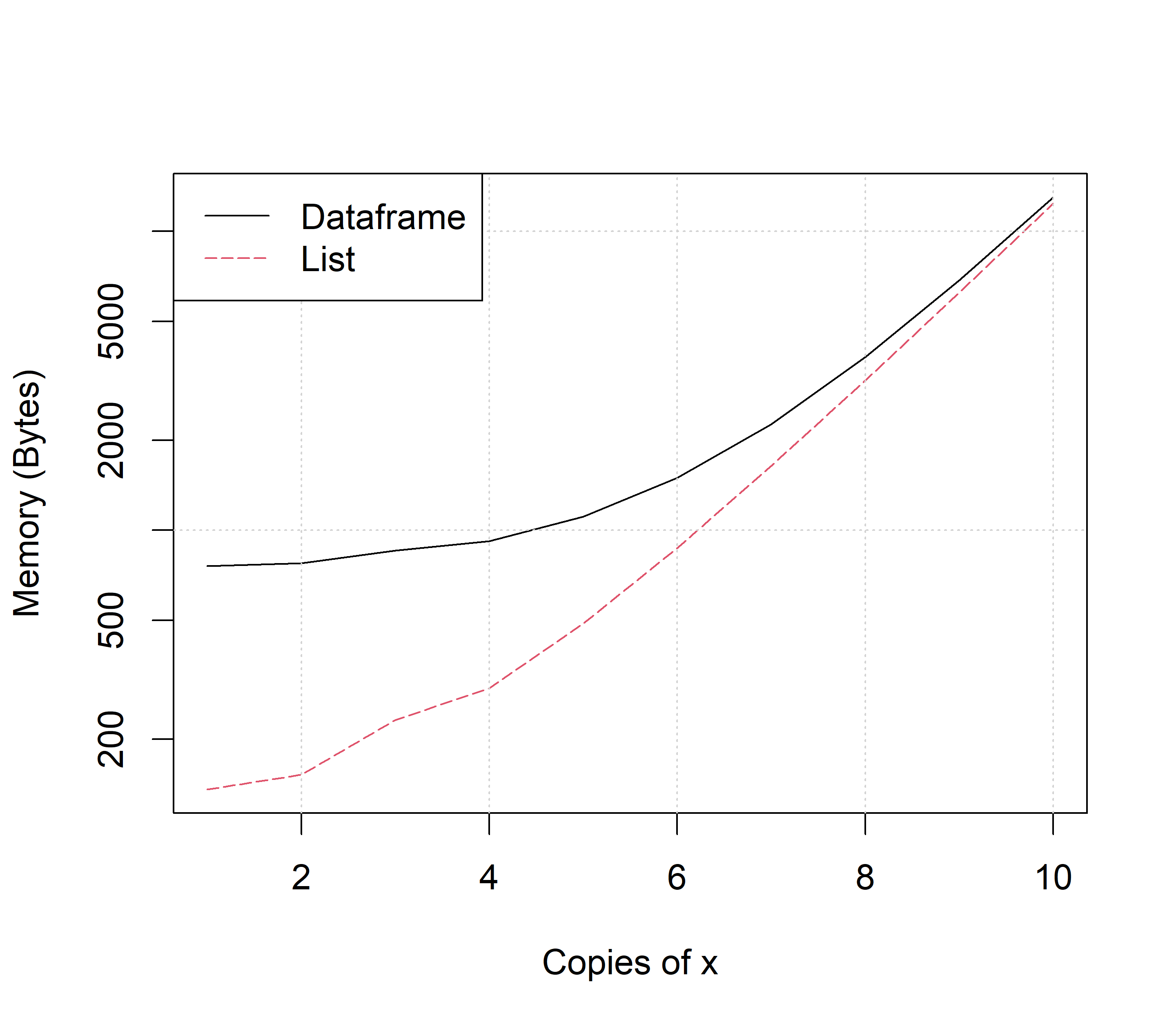
FIGURE 3.5: Comparison of list and dataframe memory useage given copies of x. Code for figure is at https://amalgamofr.org/listVSdf.R .
\(\blacksquare\)
3.9.1 Global Character Pool
R memory storage for character string objects is optimized in an unexpected way. Instead of creating addresses for user strings on the fly, R locates addresses for single immutable string values stored within a global string pool. This approach has also been called string interning (Wikipedia 2025t).
Example 3.60 \(\text{}\)
Thus, for the string below, we have the conceptual framework shown in Fig 3.6.
x <- c("a", "zyx", "PhD")![**R** character strings and the global string pool. Figure follows [@wickham2019advanced].](figs3/address4.png)
FIGURE 3.6: R character strings and the global string pool. Figure follows (Wickham 2019).
The actual pointers to the strings in the global string pool can be identified with: lobstr:ref().
ref(x, character = TRUE)█ [1:0x20f2305b828] <chr>
├─[2:0x20e9d04c0e0] <string: "a">
├─[3:0x20f1ad781f8] <string: "zyx">
└─[4:0x20f1ad782a0] <string: "PhD"> \(\blacksquare\)
String interning dramatically improves computational efficiency and decreases memory usage, because string values only need to be stored once. String pools originated with Lisp, and are also used by the Java language (Wikipedia 2025t).
3.10 Packages
An R package contains a set of related functions, documentation, data files, and other miscellany that have been bundled together. The so-called R-distribution packages are included with a conventional download of R (Table 3.3). These packages are directly controlled by the R core development team and are extremely well-vetted and trustworthy.
Packages in Table 3.4 constitute the R-recommended packages. These are not necessarily controlled by the R core development team, but are also extremely useful, well-tested, and stable, and like the R-distribution packages, are included in conventional downloads of R.
Aside from distribution and recommended packages, there are a large number of contributed packages that have been created by R-users (23680 as of 05/20/2026). Table 3.5 lists a few.
3.10.1 Package Installation
Contributed packages can be installed from CRAN (the Comprehensive R Archive Network). To do this, one can go to Packages \(>\) Install package(s) on the R-GUI toolbar (Windows), and choose a nearby CRAN mirror site to minimize download time. Once a mirror site is selected, the packages available at the site will appear. One can simply click on the desired packages to install them. Packages can also be downloaded directly from the command line using install.packages("package name"). Thus, to install the package vegan (see Table 3.5), I would simply type:
install.packages("vegan")If local web access is not available, packages can be installed as compressed (.zip, .tar) files which can then be placed manually on a workstation by inserting the package files into the library folder within the top level R directory, or into a path-defined R library folder in a user directory.
The installation pathway for contributed packages can be identified using .libPath().
[1] "C:/Users/ahoken/AppData/Local/R/win-library/4.5"
[2] "C:/Program Files/R/R-4.5.3/library"
This process can be facilitated in RStudio via applications in its Plots and Miscellany panel (see Section 2.10).
Several functions exist for updating packages and for comparing currently installed versions of packages to their latest versions at CRAN or other repositories. The function old.packages() prints a list of currently installed packages that have a (suitable) later version. Here are a few of the packages I have installed that have later versions.
head(old.packages(repos = "https://cloud.r-project.org"))[,c(1,3,4,5)] Package Installed Built ReposVer
backports "backports" "1.5.0" "4.5.2" "1.5.1"
bit64 "bit64" "4.6.0-1" "4.5.0" "4.8.2"
broom "broom" "1.0.12" "4.5.3" "1.0.13"
bslib "bslib" "0.10.0" "4.5.2" "0.11.0"
circlize "circlize" "0.4.17" "4.5.2" "0.4.18"
cli "cli" "3.6.5" "4.5.0" "3.6.6" The function update.packages() will identify, and offer to download and install later versions of installed packages.
3.10.2 Loading Packages
Once a contributed package is installed on a computer it never needs to be re-installed. However, for use in an R session, recommended packages, and installed contributed packages will need to be loaded (although see Section 2.7.1 concerning customized R startup). This can be done using the library() function, or point and click tools if one is using RStudio. For example, to load the installed contributed vegan package, I would type:
Loading required package: permuteWe see that two other packages are loaded when we load vegan: permute and lattice.
To detach vegan from the global environment, I would type:
detach(package:vegan)We can check if a specific package is loaded using the function .packages(). Most of the R distribution packages are loaded (by default) upon opening a session. Exceptions include compiler, grid, parallel, splines, stats4, and tools.
bpack <- c("base", "compiler", "datasets", "grDevices",
           "graphics", "grid", "methods", "parallel",
           "splines", "stats", "stats4", "tcltk", "tools",
           "translations", "utils")
sapply(bpack, function(x) (x %in% .packages()))
base compiler datasets grDevices graphics
TRUE FALSE TRUE TRUE TRUE
grid methods parallel splines stats
FALSE TRUE FALSE FALSE TRUE
stats4 tcltk tools translations utils
FALSE TRUE FALSE FALSE TRUE The function sapply(), which allows application of a function to each element in a vector or list, is formally introduced in Section 4.1.1.
The package vegan is no longer loaded because of the application of detach(package:vegan).
[1] FALSE
We can get a summary of information about a session, including details about the version of R being used, the underlying computer platform, and the loaded packages with the function sessionInfo().
si <- sessionInfo()
si$R.version$version.string
[1] "R version 4.5.3 (2026-03-11 ucrt)"
si$running[1] "Windows 11 x64 (build 26100)"[1] "gWidgets2tcltk" "pROC" "inline" "magrittr"
[5] "otel" "compiler" This information is important to include when reporting issues to package maintainers.
Once a package is installed its functions can generally be accessed using the double colon metacharacter, ::, even if the package is not actually loaded. For instance, the function vegan::diversity() will allow access to the function diversity() from vegan, even when vegan is not loaded.
[1] function (x, index = "shannon", groups, equalize.groups = FALSE,
[2]     MARGIN = 1, base = exp(1))
The triple colon metacharacter, :::, can be used to access internal package functions. These functions, however, are generally kept internal for good reason, and probably shouldn’t be used outside of the context of the rest of the package.
3.10.3 Other Package Repositories
Aside from CRAN, there are currently three other extensive repositories of R packages. First, the Bioconductor project (http://www.bioconductor.org/packages/release/Software/html) contains a large number of packages for the analysis of data from current and emerging biological assays. Bioconductor packages are generally not stored at CRAN. Packages can be downloaded from Bioconductor using an R script called biocLite. To access the script and download the package RCytoscape from Bioconductor, I could type:
source("http://bioconductor.org/biocLite.R")
biocLite("RCytoscape")
Second, the Posit Package Manager (formerly the RStudio Package Manager) provides a repository interface for R packages from CRAN, Bioconductor, and packages for the Python system (see Section 9.7). Third, R-forge (http://r-forge.r-project.org/) contains releases of packages that have not yet been implemented into CRAN, and other miscellaneous code. Bioconductor, Posit, and R-forge can be specified as repositories from Packages\(>\)Select Repositories in the R-GUI (Mac and Windows only), or using the repos argument in install.packages(). Other informal R package and code repositories currently include GitHub and Zenodo.
| Package | Maintainer | Topic(s) addressed by package | Author/Citation |
|---|---|---|---|
| base | R Core Team | Base R functions | R Core Team (2023) |
| compiler | R Core Team | R byte code compiler | R Core Team (2023) |
| datasets | R Core Team | Base R datasets | R Core Team (2023) |
| grDevices | R Core Team | Devices for base and grid graphics | R Core Team (2023) |
| graphics | R Core Team | R functions for base graphics | R Core Team (2023) |
| grid | R Core Team | Grid graphics layout capabilities | R Core Team (2023) |
| methods | R Core Team | Formal methods and classes for R objects | R Core Team (2023) |
| parallel | R Core Team | Support for parallel computation | R Core Team (2023) |
| splines | R Core Team | Regression spline functions and classes | R Core Team (2023) |
| stats | R Core Team | R statistical functions | R Core Team (2023) |
| stats4 | R Core Team | Statistical functions with S4 classes | R Core Team (2023) |
| tcltk | R Core Team | Language bindings to Tcl/Tk | R Core Team (2023) |
| tools | R Core Team | Tools forpackage development/administration | R Core Team (2023) |
| utils | R Core Team | R utility functions | R Core Team (2023) |
| Package | Maintainer | Topic(s) addressed by package | Author/Citation |
|---|---|---|---|
| KernSmooth | B. Ripley | Kernel smoothing | Wand (2023) |
| MASS | B. Ripley | Important statistical methods | Venables and Ripley (2002) |
| Matrix | M. Maechler | Classes and methods for matrices | Bates et al. (2023) |
| boot | B. Ripley | Bootstrapping | Canty and Ripley (2022) |
| class | B. Ripley | Classification | Venables and Ripley (2002) |
| cluster | M. Maechler | Cluster analysis | Maechler et al. (2022) |
| codetools | S. Wood | Code analysis tools | Tierney (2023) |
| foreign | R core team | Data stored by non-R software | R Core Team (2023) |
| lattice | D. Sarkar | Lattice graphics | Sarkar (2008) |
| mgcv | S. Wood | Generalized Additive Models | Wood (2011), Wood (2017) |
| nlme | R core team | Linear and non-linear mixed effect models | Pinheiro and Bates (2000) |
| nnet | B. Ripley | Feed-forward neural networks | Venables and Ripley (2002) |
| rpart | B. Ripley | Partitioning and regression trees | Venables and Ripley (2002) |
| spatial | B. Ripley | Kriging and point pattern analysis | Venables and Ripley (2002) |
| Package | Maintainer | Topic(s) addressed by package | Author/Citation |
|---|---|---|---|
| asbio | K. Aho | Stats pedagogy and applied stats | Aho (2023) |
| car | J. Fox | General linear models | Fox and Weisberg (2019) |
| dplyr | H. Wickham | Data science under the tidyverse | Wickham et al. (2019) |
| coin | T. Hothorn | Non-parametric analysis | Hothorn et al. (2006), Hothorn et al. (2008) |
| ggplot2 | H. Wickham | Tidyverse grid graphics | Wickham (2016) |
| lme4 | B. Bolker | Linear mixed-effects models | Bates et al. (2015) |
| lubridate | V. Spinu | Tidyverse dates and times | Grolemund and Wickham (2011) |
| plotrix | J. Lemon | Helpful graphical ideas | Lemon (2006) |
| spdep | R. Bivand | Spatial analysis | Bivand et al. (2013), Pebesma and Bivand (2023) |
| vegan | J. Oksanen | Multivariate analyses | Oksanen et al. (2022) |
3.10.4 Accessing Package Information
Important information concerning a package can be obtained from the packageDescription() family of functions. Here is the version of the R contributed package asbio on my work station:
packageVersion("asbio")[1] '1.13.1'Here is the version of R used to build the installed version of asbio, and the package’s build date:
packageDescription("asbio", fields="Built")[1] "R 4.5.1; ; 2026-04-22 22:18:36 UTC; windows"
3.10.5 Accessing Datasets in R-packages
The command:
data()results in a listing of a datasets available in a session from within R packages loaded in a particular R session. Whereas the code:
results in a listing of a datasets available in a session from within installed R packages.
If one is interested in datasets from a particular package, for instance the package datasets, one could type:
data(package = "datasets")All datasets in the datasets package are read into an R-session automatically, upon loading of the package. This is because the package’s dataframes were defined to be lazy loaded when the package was built (Ch 10). To access a dataset from a package that do not specify lazy loading, we must use the data() function with the data object name as an argument, after loading the data object’s package environment.
Example 3.61 \(\text{}\)
Here I load the asbio package to access its dataframe K, which contains soil potassium measurements for “identical” soils samples, from eight soil testing laboratories.
The data are now contained in a dataframe (called K) that we can manipulate and summarize.
summary(K) K lab
Min. :187 B : 9
1st Qu.:284 D : 9
Median :314 E : 9
Mean :308 F : 9
3rd Qu.:341 G : 9
Max. :413 H : 9
(Other):18 The function summary() provides the mean and a conventional five number summary (minimum, 1st quartile, median, 3rd quartile, maximum) of quantitative variables (i.e., K) and a count of the number of observations in each level of a categorical variable (i.e., lab).
\(\blacksquare\)
Example 3.62 \(\text{}\)
The Loblolly data in the datasets package does not require use of data() because of its use of lazy loading. Recall that we can access the first few rows from a dataframe using the function head():
head(Loblolly, 5)Grouped Data: height ~ age | Seed
height age Seed
1 4.51 3 301
15 10.89 5 301
29 28.72 10 301
43 41.74 15 301
57 52.70 20 301Here we apply the class() function to Loblolly. The result is surprisingly complex.
class(Loblolly)[1] "nfnGroupedData" "nfGroupedData" "groupedData" "data.frame" In addition to the dataframe class, there are three other classes (nfnGroupedData, nfGroupedData, groupedData). These allow recognition of the nested structure of the age and Seed variables (defined to height is a function of age in Seed), and facilitates the analysis of the data using mixed effect model algorithms in the package nlme (see ?Loblolly).
\(\blacksquare\)
R provides a spreadsheet-style data editor if one types fix(x), when x is a dataframe or a two dimensional array. For instance, the command fix(Loblolly) will open the Loblolly pine dataframe in the data editor (Figure 3.7). When x is a function or character string, then a script editor is opened containing x. The data editor has limited flexibility compared to software whose main interface is a spreadsheet, and whose primary purpose is data entry and manipulation, e.g., Microsoft Excel\(^{\circledR}\). Changes made to an object using fix() will only be maintained for the current work session. They will not permanently alter objects brought in remotely to a session. The function View(x) (RStudio only) will provide a non-editable spreadsheet representation of a dataframe or numeric array.
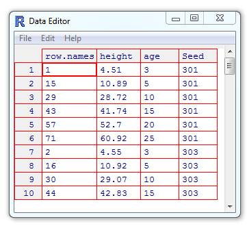
FIGURE 3.7: The default R spreadsheet editor.
3.11 Facilitating Command Line Data Entry
Command line data entry is made easier with with several R functions. The function scan() can speed up data entry because a prompt is given for each data point79, and separators are created by the function itself. Data entries can be designated using the space bar or line breaks. The scan() function will be terminated by a additional blank line or an end of file (EOF) signal. This will be Ctrl + D on Unix-likes and Ctrl + Z in Windows.
Below I enter the numbers 1, 2, and 3 as datapoints, separated by spaces, and end data entry using an additional line break. The data are saved as the object a.
Sequences can be generated quickly in R using the : operator
1:10 [1] 1 2 3 4 5 6 7 8 9 10or the function seq(), which allows additional options:
seq(1, 10) [1] 1 2 3 4 5 6 7 8 9 10
seq(1, 10, by = 2) # 1 to 10 by two[1] 1 3 5 7 9
seq(1, 10, length = 4) # 1 to 10 in four evenly spaced points[1] 1 4 7 10Entries can be repeated with the function rep(). For example, to repeat the sequence 1 through 5, five times, I could type:
[1] 1 2 3 4 5 1 2 3 4 5 1 2 3 4 5 1 2 3 4 5 1 2 3 4 5Note that the first argument in rep(), defines the thing we want to repeat and the second argument, 5, specifies the number of repetitions. I can use the argument each to repeat individual elements a particular number of times.
[1] 1 1 2 2 3 3 4 4 5 5We can use seq() and rep() simultaneously to create complex sequences. For instance, to repeat the sequence 1,3,5,7,9,11,13,15,17,19, three times, we could type:
 [1]  1  3  5  7  9 11 13 15 17 19  1  3  5  7  9 11 13 15 17 19  1  3  5  7
[25]  9 11 13 15 17 19
3.12 Importing Data Into R
As we have seen, it is possible to enter data into R at the command line; For instance, using c(). However, this will be inadvisable except for small datasets. In general, it will be much easier to import data from files saved in a plain text format. Plain text files contain readable characters, including white spaces, without formatting (e.g., absent typeface or font specifications). Plain text file content will a have a simple encoding system, allowing it to be widely recognized across different software and platforms. The most popular plain text encoding system is Unicode Transformation Format 8-bit (UTF-8), which encompasses older American Standard Code for Information Interchange (ASCII) characters (see Section 12.9). The letters (A-Z) and (a-z) are UTF-8 (and ASCII) characters (65-90) and (97-122), whereas the numbers (0-9) are UTF-8 (and ASCII) characters (48-57). On most computers, R will be able to read files with any of the 297,334 valid, assigned, UTF-8 characters:
"\u00D8, \u02AC, \u03E0, \u03BE, \U00A7, \u0100, \U00A2, \U00A3, \U00A9, \U00AE, \U00B5, \U00BA, \U00BB, \U03B8, \U03BB, \U03C0, \U03C9"[1] "Ø, ʬ, Ϡ, ξ, §, Ā, ¢, £, ©, ®, µ, º, », θ, λ, π, ω"Note Unicode characters are specified above with a backslash, \, followed by u (upper or lower case), and a specific hexadecimal (Section 12.8) code. For the sake of simplicity and portability, however, it is probably best to limit oneself to the ASCII 128 character subset, whenever possible, in data files and functions.
Plain text files can be used to store tabular data where columns (fields) are separated using a character delimiter, and rows are separated with new lines. In text files there are two possible ASCII line end characters: \n, the new-line/line-feed character, and \r, representing carriage return –named for the lever mechanism used in typewriters. Unix-likes generally use \r, whereas Windows machines use the combination \r\n, leading to potential cross-system file formatting issues.
Common tabular formats include comma separated values, which use a comma column delimiter and are often saved with a .csv extension, and white space and tab separated data files, which commonly have a .txt extension. R can read in plain text tabular data using essentially any separator format.
Important R functions for importing tabular plain text data include read.table(), read.csv(), read.delim(), and scan(). The function load() can be used to import data files in .rda data formats, or other R objects. Datasets read into R will generally be of class dataframe, with data storage mode list.
3.12.1 Import Using read.table(), read.csv(), and scan()
The read.table() function can import data organized under a wide range of formats. It’s first three arguments are very important.
-
filedefines the name of the file and directory hierarchy which the data are to be read from. -
headeris a logical (TRUEorFALSE) value indicating whetherfilecontains column names as its first line. -
seprefers to the type of data separator used for columns. Comma separated files use commas to separate columns. Thus, in this casesep = ",". Tab separators are specified as"\t". Space separators are specified as spaces, specified as simply" ".
Other useful read.table() arguments include row.names, header, and na.strings. The specification row.names = 1 indicates that the first column in the imported dataset contains row names. The specification header = TRUE, the default setting, indicates that the first row of data contains column names. The argument na.strings = "." indicates that missing values in the imported dataset are designated with periods. By default na.strings = NA.
Example 3.63 \(\text{}\)
As an example of read.table() usage, assume that I want to import a .csv file named veg.csv located in folder called veg_data, in my working directory. The first row of veg.csv contains column names, while the first column contains row names. Missing data in the file are indicated with periods. I would type:
read.table("veg_data/veg.csv", sep = ",", header = TRUE,
           row.names = 1, na.strings = ".")
Recall (section 2.6) that as a legacy of its development under Unix, R locates files in directories using forward slashes (or doubled backslashes) rather than single Windows backslashes.
\(\blacksquare\)
The read.csv() function assumes data are in a .csv format. Because the argument sep is unnecessary, this results in a simpler code statement.
read.csv("veg_data\\veg.csv", header = TRUE,
         row.names = 1, na.strings = ".")
The function scan() can read in data from an essentially unlimited number of formats, and is extremely flexible with respect to character fields and storage modes of numeric data. In addition to arguments used by read.table(), scan() has the arguments
-
whatwhich describes the storage mode of data e.g.,"logical", "integer", etc., or ifwhatis a list, components of variables including column names (see below), and -
decwhich describes the decimal point character (European scientists and journals often use commas).
Example 3.64 \(\text{}\)
Assume that veg_data/veg.csv has a column of species names, called species, that will serve as the dataframe’s row names, and 3 columns of numeric data, named site1, site2, and site3. We would read the data in with scan() using:
The empty string species = "" in the list comprising the argument what, indicates that species contains character data. Stating that the remaining variables equal 0, or any other number, indicates that they contain numeric data.
\(\blacksquare\)
The easiest way to import data, if the directory structure is unknown or complex, is to use read.csv() or read.table(), with the file.choose() function as the file argument.
Example 3.65 \(\text{}\)
For instance, by typing:
df <- read.csv(file.choose())We can now browse for a .csv files to open that will, following import, be a dataframe with the name df. Other arguments (e.g., header, row.names) will need to be used, when appropriate, to import the file correctly.
\(\blacksquare\)
Occasionally strange characters, e.g., ï.., may appear in front of the first header name when reading in files created in Excel\(^{\circledR}\) or other Microsoft applications. This is due to the addition of Byte Order Mark (BOM) characters which indicate, among other things, the Unicode character encoding of the file. These characters can generally be eliminated by using the argument fileEncoding="UTF-8-BOM" in read.table(), read.csv(), or scan().
3.12.2 Import Using RStudio
RStudio allows direct menu-driven import of file types from a number of spreadsheet and statistical programs including Excel\(^{\circledR}\), SPSS\(^{\circledR}\), SAS\(^{\circledR}\), and Stata\(^{\circledR}\) by going to File\(>\)Import Dataset. Certain restrictions may exist, however, that do not occur for read.table() and read.csv() (Table 3.6).
| CSV or Text | Excel\(^{\circledR}\) | SAS\(^{\circledR}\), SPSS\(^{\circledR}\), Stata\(^{\circledR}\) | |
|---|---|---|---|
| File system or URL imports | X | X | X |
| Change column data types | X | X | |
| Skip or include columns | X | X | X |
| Rename dataset | X | X | |
| Skip the first n rows | X | X | |
| Header row for column names | X | ||
| Trim spaces in names | X | ||
| Change column delimiter | X | ||
| Encodingselection | X | ||
| Select quote identifiers | X | ||
| Select escape identifiers | X | ||
| Select comment identifiers | X | ||
Select NA identifiers |
X | X | |
| Specify model file | X |
3.12.3 Final Considerations
It is generally recommended that datasets imported and used by R be smaller than 25% of the physical memory of the computer. For instance, they should use less than 8 GB on a computer with 32 GB of RAM.
R can handle extremely large datasets, i.e. \(> 10\) GB, and \(> 1.2 \times 10^{10}\) rows. In this case, however, specific R packages can be used to aid in efficient data handling. Parallel computing and workstation modifications may allow even greater efficiency. The actual upper physical limit for an R dataframe is \(2 \times 10^{31}-1\) elements. Note that this exceeds Excel\(^{\circledR}\) by 31 orders of magnitude (Excel\(^{\circledR}\) 2019 worksheets can handle approximately \(1.7 \times 10^{10}\) elements).
3.13 Databases
Many examples of biological data (e.g., genomes, spatial data) are extremely large and/or require multiple datasets for meaningful analyses. In this situation, storing and accessing data using a database may be extremely useful. Databases can reside locally (on a user’s computer) but more often are stored remotely and are accessed via internet links. This allows simultaneous access for multiple users, and storage of extremely large data objects. Modern databases are often structured so that data points in distinct tables can be queried, assembled, and analyzed jointly. Two common formats are Relational DataBases (RDB) and Resource Description Framework (RDF) stores (Sima et al. 2019). R can often interface with these database systems using the Structured Query Language (SQL), pronounced sequel (Chambers 2008; Adler 2010). Due to the need for additional background –provided in intervening chapters– this topic is formally introduced in Section 9.6.
Exercises
-
Create the following data structures:
- An atomic vector object with the numeric entries
1,2,3,4. - A matrix object with two rows and two columns with the numeric entries
1,2,3,4. - A dataframe object with two columns; one column containing the numeric entries
1,2,3,4, and one column containing the character entries"a","b","c","d". - A list containing the objects created in (b) and (c).
- Using
class(), identify the class and the data storage mode for the objects created in problems a-d. Discuss the characteristics of the identified classes.
- An atomic vector object with the numeric entries
-
Assume that you have developed an R algorithm that saves hourly stream temperature sensor outputs greater than \(20^\text{o}\), from each day, as separate dataframes, and places them into a list container. A
listis used because some days may have several points exceeding the threshold and some days may have none. Complete the following based on the listhi.tempsgiven below:- Combine the dataframes in
hi.tempsinto a single dataframe usingdo.call(). - Create a dataframe consisting of 10 sets of repeated measures from the dataframe
hi.temps$day2usingdo.call().
hi.temps <- list(day1 = data.frame(time = c(), temp = c()), day2 = data.frame(time = c(15,16), temp = c(21.1,22.2)), day3 = data.frame(time = c(14,15,16), temp = c(21.3,20.2,21.5))) - Combine the dataframes in
-
Given the dataframe
boobelow, provide solutions to the following questions:- Identify heights that are less than or equal to 80 inches.
- Identify heights that are more than 80 inches.
- Identify females (i.e.
F) greater than or equal to 59 inches but less 63 inches. - Subset rows of
booto only contain only data for males (i.e.M) greater than or equal to 75 inches tall. - Find the mean weight of males who are 75 or 76 inches tall.
- Use
ifelse()orif()to classify heights less than 60 inches as"small", and heights greater than or equal to 60 inches as"tall".
-
Create
x <- NA,y <- NaN, andz <- NULL.- Test for the class of
xusingx == NAandis.na(x)and discuss the results. - Test for the class of
yusingy == NaNandis.nan(y)and discuss the results. - Test for the class of
zusingz == NULLandis.null(z)and discuss the results. - Discuss
NA,NaN, andNULLdesignations what are these classes used for and what do they represent?
- Test for the class of
-
For the following questions, use data from Table 3.7 below.
- Write the data into an R dataframe called
plant. Use the functionsseq()andrep()to help. - Use
names()to find the names of the variables. - Access the first row of data using square brackets.
- Access the third column of data using square brackets.
- Access rows three through five using square brackets.
- Access all rows except rows three, five and seven using square brackets.
- Access the fourth element from the third column using square brackets.
- Apply
na.omit()to the dataframe and discuss the consequences. - Create a copy of
plantcalledplant2. Using square brackets, replace the 7th item in the 2nd column inplant2, anNAvalue, with the value12.1. - Switch the locations of columns two and three in
plant2using square brackets. - Export the
plant2dataframe to your working directory. - Convert the
plant2dataframe into a matrix using the functionas.matrix. Discuss the consequences.
- Write the data into an R dataframe called
| Plant height (dm) | Soil N (%) | Water index (1-10) | Management type |
|---|---|---|---|
| 22.3 | 12 | 1 | A |
| 21 | 12.5 | 2 | A |
| 24.7 | 14.3 | 3 | B |
| 25 | 14.2 | 4 | B |
| 26.3 | 15 | 5 | C |
| 22 | 14 | 6 | C |
| 31 | NA | 7 | D |
| 32 | 15 | 8 | D |
| 34 | 13.3 | 9 | E |
| 42 | 15.2 | 10 | E |
| 28.9 | 13.6 | 1 | A |
| 33.3 | 14.7 | 2 | A |
| 35.2 | 14.3 | 3 | B |
| 36.7 | 16.1 | 4 | B |
| 34.4 | 15.8 | 5 | C |
| 33.2 | 15.3 | 6 | C |
| 35 | 14 | 7 | D |
| 41 | 14.1 | 8 | D |
| 43 | 16.3 | 9 | E |
| 44 | 16.5 | 10 | E |
-
\(\bigstar\) Let: \[\boldsymbol{A} = \begin{bmatrix} 2 & -3\\ 1 & 0 \end{bmatrix} \text{and } \boldsymbol{b} = \begin{bmatrix} 1\\ 5 \end{bmatrix} \] Perform the following operations using R (see Section 3.1.2.1 for guidance).
- \(\boldsymbol{A}\otimes\boldsymbol{A}\)
- \(\boldsymbol{A}\odot\boldsymbol{A}\)
- \(\boldsymbol{A}\boldsymbol{b}\)
- \(\boldsymbol{b}\boldsymbol{A}\). Was there an issue? Why?
- \(det(\boldsymbol{A})\)
- \(\boldsymbol{A}^{-1}\)
-
\(\boldsymbol{A}^T\)
\(\bigstar\) We can solve systems of linear equations using matrix algebra under the framework \(\boldsymbol{A}\boldsymbol{x} = \boldsymbol{b}\), and (thus) \(\boldsymbol{A}^{-1}\boldsymbol{b} = \boldsymbol{x}\). In this notation \(\boldsymbol{A}\) contains the coefficients from a series of linear equations (by row), \(\boldsymbol{b}\) is a vector of solutions given in the individuals equations, and \(\boldsymbol{x}\) is a vector of solutions sought in the system of models. Thus, for the linear equations:
\[\begin{aligned} x + y &= 2\\ -x + 3y &= 4 \end{aligned}\]
\[\boldsymbol{A} = \begin{bmatrix} 1 & 1\\ -1 & 3 \end{bmatrix}, \boldsymbol{ x} = \begin{bmatrix} x\\ y \end{bmatrix}, \text{ and } \boldsymbol{b} = \begin{bmatrix} 2\\ 4 \end{bmatrix}.\]
\[\boldsymbol{A}^{-1}\boldsymbol{b} = \boldsymbol{x} = \begin{bmatrix} 1/2\\ 3/2 \end{bmatrix}.\]
using R (see Section 3.1.2.1 for guidance).
\[ \begin{aligned} 3x + 2y - z &= 1\\ 2x - 2y + 4z &= -2\\ -x + 0.5y -z &= 0 \end{aligned} \]
-
Complete the following exercises concerning the R contributed package asbio:
- Install80 and load the package asbio for the current work session.
- Access the help file for
bplot()(a function in asbio). - Load the dataset
fly.sexfrom asbio. - Obtain documentation for the dataset
fly.sexand describe the dataset variables. - Access the column
longevityin fly.sex using the functionwith().
Create .csv and .txt datasets, place them in your working directory, and read them into R.
How does R uses symbols? Create a symbol and explain its characteristics.
-
Create the lists
list1 <- list(a = c(1, 2, 3), b = c("a", "b")); list2 <- list1.- Show that the lists and contents of these lists have the same addresses using
lobstr::rep(). - Modify
list2by runninglist2$c <- "stuff". What happened to the addresses oflist1andlist2and their contents? Use the term copy-on-modify correctly in your answer.
- Show that the lists and contents of these lists have the same addresses using
-
Create an object containing a 1000 random outcomes,
x, and a list,listob, containingx, usingx <- runif(10^3); listob <- list(x).- Find the size of
xandlistobusinglobstr::obj_size(). - Create
listob2 <- list(x, x, x, x). Explain why the memory size oflistobandlostob2are so similar despite the fact thatlostobcontains one copy ofx, andlostob2contains four.
- Find the size of
Define the term global character pool.