2 Some Basics
“Learning to write programs stretches your mind, and helps you think better."
- Bill Gates, 1955-
2.1 First Steps
Starting R in Windows will open the R Graphical User Interface (R-GUI) and console (Fig 2.1). Two things will appear in the console: the license disclaimer (blue text at the top of the console), and the command line prompt, \(\boldsymbol{>}\). The prompt indicates that R is ready for a command. All commands in R must begin at \(\boldsymbol{>}\).
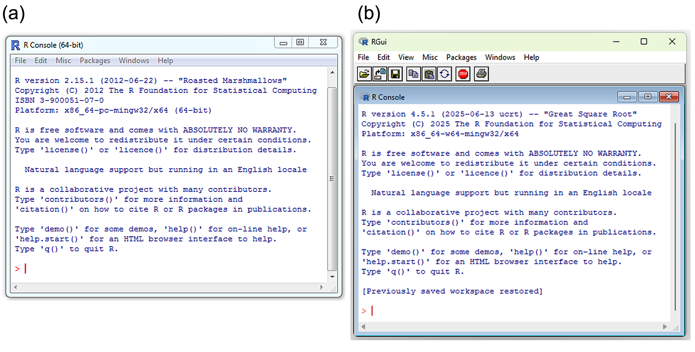
FIGURE 2.1: R-GUIs for Windows: (a) an older edition of R, ver. 2.15.1, ‘Roasted Marshmallows’, ca. 2012, and (b) a more recent (2025) edition of R, ver 4.5.1, ‘Great Square Root’.
The default appearance of the R-GUI will vary slightly among operating systems22. In Windows, the command line prompt and user commands are colored red (Fig 2.1), and output, including errors and warnings, are colored blue. In Mac OS, the command line prompt will be purple, user inputs will be blue, and output will be black (Fig 2.2a).
A Linux R-GUI, similar to those in Windows and Mac OS, can be implemented by opening R from a system shell (Section 9.2) with the command R -g Tk &. In this setting, the command line prompt, user commands, and output will all be colored black (Fig 2.2b).
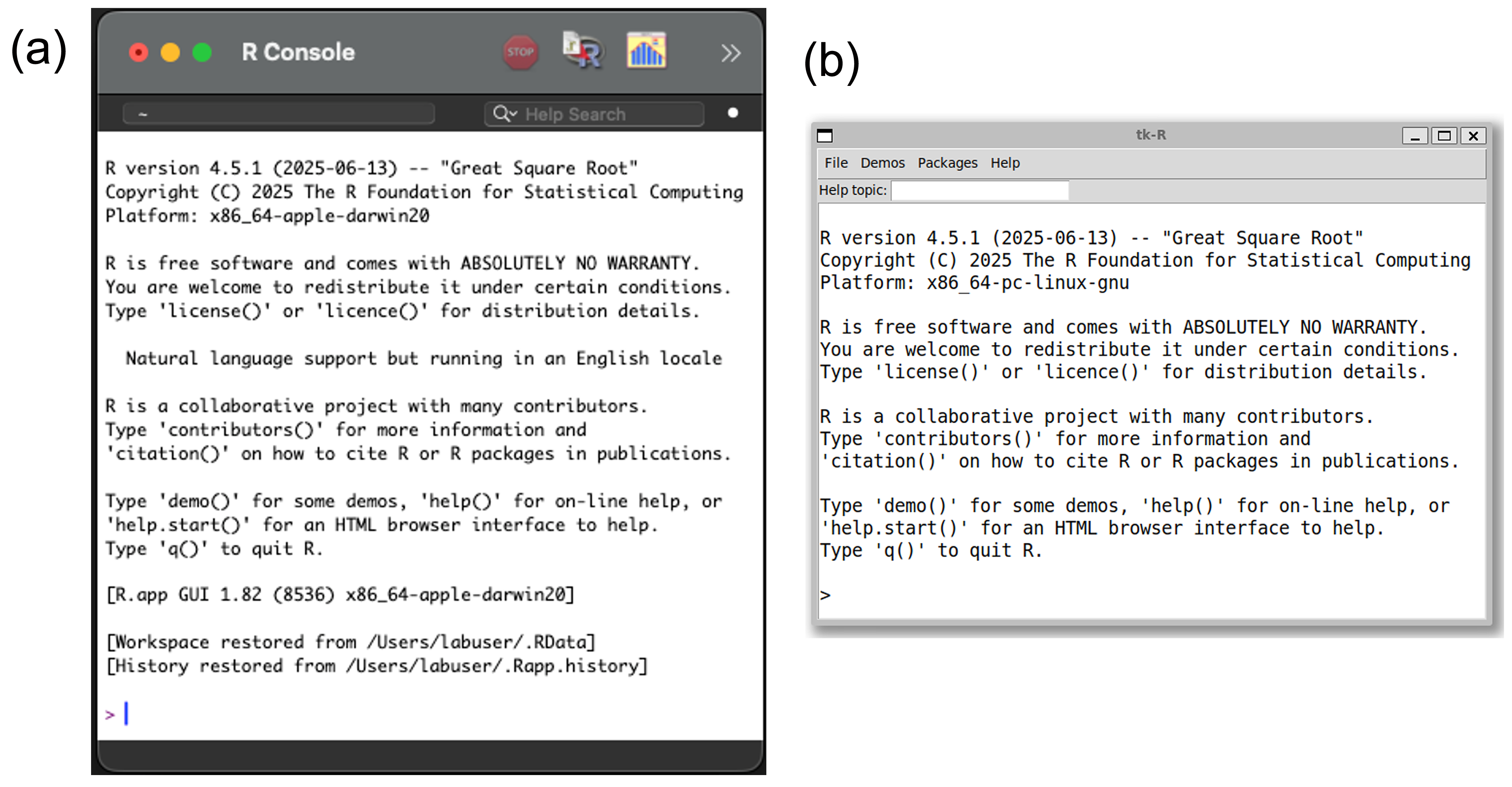
FIGURE 2.2: R-GUIs for recent versions of R, ver. 4.5.1 ‘Great Square Root’ in (a) Mac OS, and (b) Linux/Ubuntu. The Linux GUI was prompted at a terminal with R -g Tk &.
A GUI-less implementation of R can be called from a terminal shell in Windows (e.g., cmd or PowerShell, Section 9.2), Mac OS, or Linux23, by simply typing R or R.exe at the command line. This will begin an interactive R session within the system terminal itself (Fig 2.3)24.
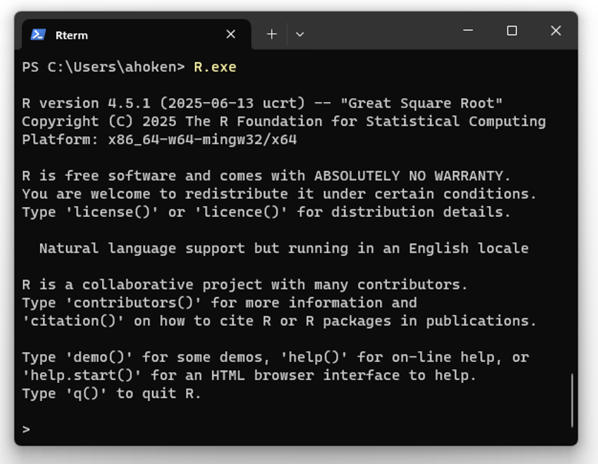
FIGURE 2.3: The Rterm (R-terminal) shell, implemented from a Windows PowerShell terminal with the command R.exe. To access PowerShell, press the Windows key, 🪟, type powershell, and press Enter.
We can exit R at any time by typing q() in the console. From R-GUIs we can close the GUI window, or select Exit (Windows), Close (Mac-OS) or Quit (Linux) from respective File pulldown menus.
2.2 First Operations
As an introduction we can use R to evaluate a simple mathematical expression. Type 2 + 2 and press Enter.
2 + 2[1] 4The output term [1] means, “this is the first requested element.” In this case there is just one requested element, 4, the solution to 2 + 2. If the output elements cannot be held on a single console line, then R would begin the second line of output with the element number comprising the first element of the new line. For instance, the command rnorm(20) will generate 20 pseudo-random samples25 from a standard normal distribution (see Ch 3 in Aho (2014)). We have:
rnorm(20) [1] 1.1447858 -1.7545477 0.1864832 -0.0641109 -1.3307695 -1.0349850
[7] 0.8016181 0.2828213 0.6304495 1.0085684 0.7985790 1.6940464
[13] 0.5851900 -1.2983055 -1.4693586 -1.1619698 0.2281920 -1.0543901
[19] 0.2935940 1.2532395The reappearance of the command line prompt indicates that R is ready for another command. Multiple commands can be entered on a single line separated by semicolons, although this may decrease code readability.
2 + 2; 3 + 2[1] 4[1] 5R commands are generally insensitive to white spaces, including tabs. This allows the use of spaces to make code more legible. To my eyes, the command 2 + 2 is simply easier to read (and potentially debug) than 2+2.
2.2.1 Use Your Scroll Keys
As with many other command line environments, the scroll keys (Fig 2.4) provide an important shortcut in R. Instead of editing a line of code by tediously mouse-searching for an earlier command to copy, paste and then modify, you can simply scroll back through your earlier work using the upper scroll key, i.e., \(\uparrow\) . Accordingly, scrolling down using \(\downarrow\) will allow you to move forward through earlier commands.

FIGURE 2.4: Typical scroll direction keys on a keyboard.
2.2.2 Note to Self: #
R will not recognize commands preceded by #. As a result this is a good way for us to leave messages to ourselves.
# Note at beginning of line
2 + 2
[1] 4We can even place comments in the middle of an expression, as long the expression is finished on a new line.
2 + # Note in middle of line
+ 2
[1] 4In the “best” code writing style it is recommended that one place a space after # before beginning a comment, and to insert two spaces following code before placing # in the middle of a line. This convention is followed above.
2.2.3 Unfinished Commands
R will be unable to move on to a new task when a command line is unfinished. For example, type
and press Enter. We note that the continuation prompt, +, is now where the command prompt should be. R is telling us the command is unfinished.
The easiest and most portable way to interrupt the continuation prompt in R-GUIs is by pressing Esc (all OS). One can also return to the command prompt by finishing the unfinished expression, clicking Misc \(>\) Stop current computation or Misc \(>\) Stop all computations from the R-GUI toolbar (Windows only)26, clicking on the menu stop button, 🛑, (Windows and Mac OS only; Figs 2.1, 2.2a), or typing Ctrl + C (Linux terminal).
2.3 Keyboard Shortcuts
R contains a number of useful keyboard shortcuts. For example, it may be evident that the R-console can quickly become cluttered and confusing. To clear the console (without actually deleting stored work from a session), press Ctrl + L or, from the Edit pulldown menu, click Clear console (non-Linux only). A full list of keyboard shortcuts can be obtained by typing: Alt + Shift + K (Windows and Linux) or Option + Shift + K (Mac OS). Keyboard shortcuts can be customized (or created), if one is running R from a sophisticated IDE like RStudio (Section 2.10).
2.4 R Objects
In computer programming, an object is an identifiable, dynamically generated, data container. Objects can be assigned human-readable names and will possess implicit or explicit attributes, including structural frameworks called classes (Section 2.4.7)27. A frequently used maxim (adopted from S) is: “everything in R is an object” (Chambers 2008).
2.4.1 Expression and Assignments
Object processes in R will be managed as expressions or assignments. If a process is an expression, it will be evaluated, printed, and discarded. Examples include: 2 + 2. Conversely, an assignment evaluates an expression, and binds the output to a name. To generate an object assignment, we use the assignment operator: <-. The operator represents an arrow that “points” toward the user-defined name.
Example 2.1 \(\text{}\)
For example, to label the result of 2 + 2 as y, I can type:
y <- 2 + 2The code y <- 2 + 2 literally means: “2 + 2 is bound to the name y”28.
The assignment operator can go on either side of an expression. Thus, as an alternative, I could have typed:
2 + 2 -> yThe leftward assignment operator, <-, is generally used instead of the rightward, ->, because it is often easier to conceptualize the relationship object_name <- object.
\(\blacksquare\)
The results of an assignment are not automatically printed. That is, the operation y <- 2 + 2 will not elicit an apparent response from R. However, to print y (to see the value bound to the name y), I can simply type y or print(y)29.
\(\blacksquare\)
The mathematical equals operator, =, can also be used as an assignment operator. Like <-, = assigns from right to left.
Example 2.3 \(\text{}\)
For instance,
y = 2 + 2
y
[1] 4\(\blacksquare\)
The equals sign has limited applicability as an assignment operator, compared to <-30. Thus, in this document, I use <- for object assignments, and save = for specifying arguments in R functions (Section 2.4.3).
Once assigned, one can call y directly for appropriate operations in R.
Example 2.4 \(\text{}\)
Because of the numeric character of y, I could do something like:
3 * log(y) # log() is the natural log [1] 4.158883\(\blacksquare\)
2.4.2 Character Strings
R objects need not be numeric. In computer programming, a character string or string is a collective sequence of characters representing text31. Character strings in R are delimited with quotes: " " or ' '.
Example 2.5 \(\text{}\)
Here I bind the name y to a well-known character string.
y <- "Hello, world!"; y[1] "Hello, world!"
y <- 'Hello, world!'; y [1] "Hello, world!"The presence of two types of quote operators allows one to make quotes part of a string:
"'Hello', world!"[1] "'Hello', world!"\(\blacksquare\)
2.4.3 Functions and their Arguments
Importantly, the script print(y) in Example 2.2 provides one of our first clear uses of a special type of R object called a function. Functions underlie essentially every R process (Chambers 2008).
R functions generally require a user to specify arguments that direct and control its behavior. Argument names and their assigned values are stipulated within parentheses, following the function name. Thus, we would use the following framework for calling an R function: function.name(argument1, argument2, argument3, etc).
For the most common family of R functions (closure functions), one can obtain a list of arguments and their default values using the function formals().
Example 2.6 \(\text{}\)
For example,
formals(print)$x
$...The first argument in print(), x, refers to the name of the object to be printed. This is only argument required by print(). The second argument is the so-called triple dot placeholder, .... This (optional) argument allows additional arguments to be passed from various printing methods that can be called using the generic function name print() (see Section 8.7).
\(\blacksquare\)
Arguments in R functions can be set by users in two ways.
- One can provide acceptable values for arguments, in the order that the arguments occur in the list reported by
formals(). For example, for the functiona_function, if I wish to assign the valuesxandyto the first and second arguments, respectively, I could type:a_function(x, y). - One can refer to an argument by its name, and specify values for the argument using the
=operator. That is, for some functiona_function, with some argumentsfooandbar, that I wish to assign the valuesxandy, I could type:a_function(foo = x, bar = y). This approach should be used if one does not remember the order of arguments in a function (if you don’t remember whetherfoois the first or fifth argument), or if one wishes to change/specify only certain arguments from a large number of arguments.
Example 2.7 \(\text{}\)
Under approach 2, we can print the object y, created in Example 2.5, by typing:
print(x = y)[1] "Hello, world!"Of course, data object names other than y can be supplied to the argument x in print(). For example, to print an object named z, I could use either print(z) or print(x = z).
\(\blacksquare\)
One can maintain the default value for an argument by simply ignoring that argument in the function call. For example, if a_function, has argument defaults foo = x, bar = y, and I wished to change the value of foo to baz, while maintaining the default value for bar, I could type: a_function(foo = baz). Occasionally, a function’s defaults will allow it to run without user value specifications for any arguments. In this case, I could run a_function by typing: a_function().
2.4.4 Naming Objects
When binding an R-object to a name, we should try to keep the name simple, and avoid names that already represent important definitions and functions. The names TRUE, FALSE, NULL, NA, NaN, and Inf are reserved by R. Additionally, we cannot have names:
- beginning with a numeric value,
- containing spaces, colons, or semicolons,
- containing mathematical operators (e.g.,
*,+,-,^,/,=), - containing important R metacharacters (e.g.,
@,#,?,!,%,&,|).
However, even these “forbidden” names and characters can be used if one encloses them in backticks` `, also called accent grave characters. For example, the code, `?` <- 2 + 2 will create an object named `?`, containing the number 4.
Names should, if possible, be descriptive. Thus, for an object containing 20 random observations from a normal distribution, the name rN20 may be superior to the easily-typed, but anonymous name, x. Finally, we should remember that R is case sensitive. That is, each of the following \(2^4\) combinations will be recognized as distinct: name, Name, nAme, naMe, namE, NAme, nAMe, naME, NaMe, nAmE, NamE, naME, NAMe, nAME, NaME, NAmE, NAME.
2.4.5 Listing Objects
The lexical scoping characteristics of R (Section 1.4.1.2) have important consequences when considering objects and their names. An object’s name will be assigned to a particular R environment, a specialized storage system whose features are formally considered in Ch 8. By default, an object will be assigned by R to the environment where it was defined/created, although this can be modified.
Only objects in the current environment can be directly accessed by calling their names32. The current environment will be reported by the function environment().
Example 2.8 \(\text{}\)
The R session itself is defined to be the so-called global environment: .GlobalEnv.
<environment: R_GlobalEnv>\(\blacksquare\)
A list of objects assigned to particular environments can be obtained using the functions objects() or ls(). By default, object searches from objects() and ls() are limited to the current environment which, from the perspective of the processes generating this document (Section 2.10.2), is the global environment.
Example 2.9 \(\text{}\)
Currently, I only have the object y (which has been applied and modified several times) in GlobalEnv.
objects()[1] "y"Note that in the previous and current example I run environment() and objects() without arguments.
\(\blacksquare\)
2.4.6 Combining Data
To combine a collection of numbers or other data into a single entity, one can use the important R function c(), which means “combine”.
Example 2.10 \(\text{}\)
To define the numbers 23, 34, and 10 collectively to be an object named x, I would type:
x <- c(23, 34, 10)We could then do something like:
x + 7[1] 30 41 17Note that seven was added to each element in x.
\(\blacksquare\)
2.4.7 Object Classes
Under the idiom of object oriented programming (OOP)33, a class is an attribute that imparts a common structure to all objects belonging to the same class type. Class types will generally have associated method functions specifically suited for the characteristics of their objects (e.g., specific functions for plotting, printing, etc.).
Some common R object classes are shown in Table 2.1, along with several new functions used to create objects with those classes, including: raw(), expression(), list(), factor(), function(), matrix(), array(), and data.frame(). We will learn about these functions, and create objects representing all of these classes over the next few chapters. We will also learn how to create our own personalized classes and associated methods (Section 8.7).
| Class | Example |
|---|---|
logical |
x <- TRUE |
integer |
x <- 1L |
numeric |
x <- 1 |
complex |
x <- 5i |
character |
x <- "a" |
list |
x <- list() |
expression |
x <- expression(x * 4) |
raw |
x <- raw(2) |
factor |
x <- factor("a","a","b") |
function |
x <- function(y)y + 1 |
matrix |
x <- matrix(nrow = 2, rnorm(4)) |
array |
x <- array(rnorm(8), c(2, 2, 2)) |
data.frame |
x <- data.frame(v1 = c(1,2), v2 = c("a","b")) |
R objects will always have at least one class identifiable with the function class().
class(x)[1] "numeric"Objects in class numeric (and those from several other widely-used classes) can be evaluated mathematically.
2.4.8 Object Base Types
In programming, base types or primitive types are fixed, internal, definitions for particular kinds of data. Every R object will have a single base type34. In R, a base type will correspond to a specific underlying C language structure called an SEXPTYPE, meaning S-expression (SEXP) type (R Core Team 2024a). A lack of knowledge concerning C SEXPTYPEs will not prevent one from using R effectively. A working knowledge of associated R base types, however, is crucial for understanding how R works. Additional information concerning the workings of R SEXPTYPEs is provided in Appendix B.
There are currently 24 R base types, and each has a unique, corresponding C SEXPTYPE (Table 2.2). New base types are added/modified only occasionally by the R-core team, because of the large effort required to reprogram R at a fundamental level (Wickham 2019)35.
| Base type | Example | Application | SEXPTYPE |
|---|---|---|---|
logical |
x <- TRUE |
atomic vector (logical) | LGLSXP |
integer |
x <- 1L |
atomic vector (integer) | INTSXP |
double |
x <- 1 |
atomic vector (double) | REALSXP |
complex |
x <- 1i |
atomic vector (complex) | CPLXSXP |
character |
x <- "a" |
atomic vector (character) | STRSXP |
raw |
x <- raw(2) |
atomic vector (raw bytes) | RAWSXP |
list |
x <- list() |
general (list) vector | VECSXP |
expression |
x <- expression(x * 4) |
expression vector | EXPRSXP |
NULL |
x <- NULL |
NULL | NILSXP |
environment |
x <- globalenv() |
environment | ENVSXP |
symbol |
x <- quote(a) |
language component | SYMSXP |
language |
x <- quote(a + 1) |
language component | LANGSXP |
pairlist |
x <- formals(mean) |
language component | LISTSXP |
S4 |
x <- stats4::mle(function(x=1)x^2) |
non-simple object | OBJSXP |
any |
No example | C-internal | ANYSXP |
bytecode |
No example | C-internal | BCODESXP |
promise |
No example | C-internal | PROMSXP |
... |
No example | C-internal | DOTSXP |
weakref |
No example | C-internal | WEAKREFSXP |
externalptr |
No example | C-internal | EXTPTRSXP |
char |
No example | C-internal | CHARSXP |
The meaning and use of some of the base types may seem clear, for instance integer and character, which are also class designations (Table 2.1). Most of the base types are specifically addressed in later chapters, including list, complex, logical, integer, NULL, and symbol (Ch 3), character and language (Chs 4 and 5), closure, special, builtin, environment, pairlist, S4, and promise (Ch 8) and raw and double (Ch 12). Base types meant for C-internal processes, i.e., object, any, bytecode, promise, ..., weakref, externalptr, and char, are not easily accessible with R source code (R Core Team 2024b).
Base types can be identified using the function typeof().
Example 2.11 \(\text{}\)
For example, for our latest version of x (from Example 2.10), we have:
typeof(x)[1] "double"Base types of numeric objects define their internal storage mode, i.e., the way R caches their values in primary memory37. We see that x has storage mode double, meaning that its numeric values are stored with double precision, generally requiring 64 bits in computer memory, and resulting in recognizable and distinguishable values between approximately \(5 \times 10^{-323}\) and \(2 \times 10^{307}\) (Section 12.7).
The R session itself (the global environment) has base type environment:
typeof(.GlobalEnv)[1] "environment"
\(\blacksquare\)
2.4.9 Object Attributes
All R-objects, except those of base type NULL (Section 3.6.3), can be assigned attributes, including dimensions for tabular array formats, and names, which can be used to label object elements (e.g., columns in an R dataframe, Section 3.1.4). Object attributes can be tracked with attributes().
Example 2.12 \(\text{}\)
Some attributes will be added automatically to R objects, because of their class. Typing:
attributes(x)NULLindicates that x (as defined in Example 2.10) does not have attributes. However, using coercion (Section 3.5) we can convert x to an object of classes matrix and array (see Section 3.1.3.1).
[1] "matrix" "array"
attributes(x)$dim
[1] 3 1Now x has the attribute dim (i.e., dimension). Specifically, x is a three-celled matrix. It has three rows and one column.
\(\blacksquare\)
Object attributes can be set (and tracked) using the function attr().
Example 2.13 \(\text{}\)
Here I modify the dimension attribute of x:
Now x has three columns and one row.
attributes(x)$dim
[1] 1 3
x [,1] [,2] [,3]
[1,] 23 34 10\(\blacksquare\)
Amazingly, underlying object characteristics allow R to simultaneously store and distinguish objects with the same name.
Example 2.14 \(\text{}\)
For instance:
[1] 6[1] 6In general, it is not advisable to name an object after a frequently used function. Nonetheless, the function sum(), which calculates the sum of a collection of numeric data (Section 2.9.7), is distinguishable from the new user-created object sum, because these objects have different underlying characteristics (e.g., base types and environments). We can remove the user-created object sum, with the function rm(). This leaves behind only the function sum(), which I print below:
rm(sum)
sum
function (..., na.rm = FALSE) .Primitive("sum")\(\blacksquare\)
The capacity of R to track and distinguish names and their corresponding objects, including functions, is a primary focus of Section 8.8.
2.4.10 \(\bigstar\) Explicit and Implicit Classes and R-OOP
In R, a class can be viewed as a potential object attribute. If attr(x "class") does not return one or more class for x, this means that an explicit class (for example, one assigned through user-directed explicit coercion, Section 3.5) does not exist for x. In this case, R will assign an implicit class to x, based on an object’s user-defined structure, its base type, or rarely, mode(x). Frequently assigned implicit classes include matrix, array, function and numeric. As a general programming rule, implicit classes make computational processes simpler, but are less predictable and more difficult to debug than explicit class operations.
Implicit coercion often occurs as R attempts to fulfill a user-requested operation.
Example 2.15 \(\text{}\)
For example,
sum(TRUE, FALSE, TRUE)[1] 2
The outcome 2 is returned by sum() (which takes the sum of values in its arguments) because R implicitly coerces logical outcomes to have base type integer (where TRUE = 1, FALSE = 0), because the requested operation required numeric outcomes.
\(\blacksquare\)
Example 2.16 \(\text{}\)
Consider the character object x below:
x <- c("a","b","c")
typeof(x)[1] "character"
class(x)[1] "character"
attr(x, "class")NULLConfusingly, class(x) indicates that x has a class, whereas attr(x, "class") indicates that it doesn’t (outcome = NULL).
The object x above is an atomic vector (Table 2.2, Section 3.1.1) containing strings. Atomic vectors comprise the simplest (and oldest) building blocks for R data objects, and will have no explicit attributes (including classes). Thus, while an implicit class has been assigned to x (identifiable with class(x)), an explicit class (identifiable with attr(x, "class")) has not.
Below I try to assign x to the class numeric using attr().
[1] "numeric"
class(x)[1] "numeric"However, this merely adds confusing metadata. It does not change the data storage mode of x. That is, unlike logical outcomes, string outcomes in x are not implicitly converted to numbers.
sum(x)Error in `sum()`:
! invalid 'type' (character) of argumentAlthough, this is reasonable (it is unclear how one could create rules to convert strings to numbers), it also reveals the potential inconsistency of implicit coercion. To explicitly change the data storage mode of an R object x, one must use explicit coercion functions like as.numeric() (see Section 3.3), not attr(x, "class").
\(\blacksquare\)
Idiosyncrasies in the explicit and implicit assignment of object classes have a historic basis, and distinguish R from other OOP languages. Wickham (2019) considers this by recognizing two types of R objects: base and OO.
- The first version of R was intended to emulate S version 3 (S3) (Ihaka 1998). S3, however, incorporated older object definitions (from S1 and S2) that existed before anyone considered the need for an S OOP system (Chambers 2008). These objects, which also wound up in R, can be considered base objects (Wickham 2019). Base objects, which include atomic vectors (Table 2.2), will be assigned (by R) to an implicit class, so that they can be evaluated and handled. They will not, however, have explicit attributes, including classes. As a result, for a base object
x,attr(x, "class")will returnNULL. -
OO objects comprise a newer, object-oriented, framework for R objects. Unlike base objects, an OO object
xwill promptattr(x, "class")to return at least one class assignment. Several approaches, including S3 and S4 (named after the versions of S that they originated from), along with other approaches, can be used to create new OO classes and associated methods in R. This topic is considered in Sections 8.7.1 and 8.7.2.
The operation class(x) will return either an implicit or an explicit class type depending on whether x is a base or OO object, respectively.
2.5 Getting Help
There is no single perfect source for information/documentation for all aspects of R. Detailed manuals from CRAN are available concerning the R language definition, basic operations, and package development. These resources, however, often assume a familiarity with Unix-like operating systems and computer science terminology. Thus, they may not be particularly helpful to biologists, raised on Windows, who are new to R.
2.5.1 help() and ?
A comprehensive help system is available for many R components including operators, and loaded package dataframes and functions. The system can be accessed via the question mark, ?, operator and the function help().
Example 2.17 \(\text{}\)
For instance, if I wanted to know more about the plot() function, I could type:
?plotor
help(plot)\(\blacksquare\)
Documentation for packaged R functions (Section 3.10) must include an annotated description of function arguments, along with other pertinent information, and documentation for packaged datasets must include descriptions of dataset variables38. The quality of documentation will generally be excellent (though succinct) for functions from packages in the default R download (i.e., the R-distribution packages, see Section 3.10), but will vary from package to package otherwise.
For help and documentation concerning programming metacharacters used in R (for instance @, #, ?, !, %, &, |), one would enclose the metacharacters with quotes. For example, to find out more information about the logical operator & I could type help("&") or ? "&". Placing two question marks in front of a topic will cause R to search for help files with respect to all packages in a workstation.
Example 2.18 \(\text{}\)
For instance, type:
??lmor, alternatively
help.search(lm)for a huge number of help files on linear model functions identified with fuzzy matching39.
\(\blacksquare\)
Help for particular R-questions can often be found online using the search engine at http://search.r-project.org/. This link is provided in the Help pulldown menu in the R console (non-Linux only). Helpful online discussions can also be found at Stack Overflow, and Stats Exchange. Emerging (though often unreliable) guides for programming include AI Large Language Models (LLMs) from search engines like Google.
2.5.2 demo() and example()
The function demo() allows one access to coded examples that developers have worked out for a particular function or topic. For instance, type:
demo(graphics)for a brief demonstration of R graphics. Typing
demo(persp)will provide a demonstration of 3D perspective plots. And, typing:
demo(Hershey)will provide a demonstration of available modifiable symbols from the Hershey family of fonts (see Ch 6 in Hershey (1967)). Finally, typing:
demo()lists all of the demos available in the loaded libraries for a particular workstation. The function example() usually provides less involved demonstrations from the man package directories (short for user manual, see Ch 10) in an R package. For instance, type:
example(plotmath)for a coded demonstration of mathematical graphics.
2.5.3 Vignettes
R packages often contain vignettes. These are short documents that generally describe the theory underlying algorithms and guidance on how to correctly use package functions. Vignettes can be accessed with the function
vignette(). To view all vignettes for all installed packages (Section 3.10.1), type:
vignette(all = TRUE)To view all vignettes available for loaded packages (see Section 3.10.2), type:
vignette(all = FALSE)To view vignettes for the R contributed package asbio (following its installation), type:
vignette(package = "asbio")To see the vignette simpson in package asbio, type:
vignette("simpson", package = "asbio")The function browseVignettes() provides an HTML-browser that allows interactive vignette searches.
2.6 The Working Directory
A working directory greatly simplifies programmatic operations by defining a specific default address for acquiring and sending files. Unless changed, the R working directory is set to be the home directory of your computer. In Windows, one can print the user home directory (i.e., R_USER) with:
Sys.getenv("R_USER")[1] "C:/Users/ahoken/Documents"The function Sys.getenv() can be used to obtain paths and definitions for R environment variables (Section 2.7.1.2)
For instance, here is the home path (R_HOME) for the version of R currently being used:
Sys.getenv("R_HOME")[1] "C:/PROGRA~1/R/R-45~1.3"The command getwd() shows the file path for the current working directory.
Example 2.19 \(\text{}\)
Here is the working directory of this (GitHub-linked) manuscript.
getwd()[1] "C:/Users/ahoken/Documents/GitHub/Amalgam"\(\blacksquare\)
The working directory can be changed with the command setwd(filepath), where filepath is the location of the desired directory, or by using pulldown menus, i.e., File \(>\) Change dir (non-Linux only). Because R developed under Unix, we must specify directory hierarchies using forward slashes or by doubling backslashes.
Example 2.20 \(\text{}\)
To establish a working directory file path to the Windows directory:
C:\Users\User\Documents, I would type:
setwd("C:/Users/User/Documents")or
setwd("C:\\Users\\User\\Documents")\(\blacksquare\)
2.7 Options
To enhance an R session, we can adjust the appearance of the R-console and customize options that affect expression output. These include the characteristics of the graphics devices, the width of print output in the R-console, and the number of print lines and print digits. Changes to some of these parameters can be made by going to Edit \(>\) GUI Preferences in the R-toolbar. Many other parameters can be changed using the options() function. To see all alterable options one can type:
options()The resulting list is extensive. To modify options, one would simply define the desired change within parentheses following a call to options. For instance, to see the default number of digits in printed output, I would type:
options("digits")$digits
[1] 7To change the default number of digits from 7 to 5 in the current session, I would type:
options(digits = 5)
pi # = irrational constant pi
[1] 3.1416One can revert back to default options by restarting an R session or by saving defaults as an object, and implementing them. For instance:
One can set particular R options to be used in every R session by defining them in .Rprofile and .Renviron files (next Section).
2.7.1 \(\bigstar\) Advanced Start-up Options
R start-up procedures are rather complex and reflect R’s origins under Unix networks. One can completely ignore these protocols with little effect on performance. A basic understanding of the procedures, however, allows a great deal of personalized control over R.
Upon start-up, R will silently run files named .Rprofile, .Renviron, and files with .Rhistory and .Rdata extensions, that are housed in the user home directory (i.e., R_USER), the directory R_HOME/etc, and the current working directory. For complete details, see Appendix B. .Rprofile and .Renviron are considered below. .Rhistory and .Rdata files are formally introduced in Sections 2.8.1 and 2.8.2, respectively.
2.7.1.1 .Rprofile
One can use .Rprofile files to set persistent session options, load installed packages, define a favorite package repository (Section 3.10), and even create aliases and defaults for frequently used functions.
In Windows, a site-wide R profile file named Rprofile.site will be located in your R_HOME/etc directory following a conventional download. The file will contain some simple commented options, written as R scripts, that one can readily modify. Additional .Rprofile files can be placed in the user home directory, or in a working directory (Section 2.6). R will check for these and run them after running the .Rprofile.site file (Appendix C).
Example 2.21 \(\text{}\)
Here is the content of one of my current .Rprofile files.
options(repos = structure(c("http://ftp.osuosl.org/pub/cran/")))

if (interactive()){
  .First <- function(){
  library(asbio)
  cat("\nWelcome to R Ken! ", date(), "\n")
  }
  .Last <- function(){
  cat("\nGoodbye Ken", date(), "\n")
  }
}
The repos command in options (Line 1) defines my preferred CRAN repository mirror site (see Section 3.10). The function .First( ) (Lines 4-7) will be run at the start of the R session and .Last( ) (Lines 8-10) will be run at the end of the session. R functions will be formally introduced in Ch 8.
As we go through this book it will become clear that Lines 4-10 prompt R to say “Hello”, load the package asbio (R packages are formally considered in Section 3.10), print the date/time (using the function date()) when R opens, and say “Goodbye”, and print the date/time, when R closes. Note that I nest .First( ) and .Last( ) within the command interactive() (Line 2), which returns TRUE (Section 3.2), if R is being run interactively (with an assumed human operator) –allowing the subsequent code to be run. Clearly there is no need to say “Hello” or “Goodbye” if interactive() returns FALSE.
\(\blacksquare\)
2.7.1.2 .Renviron
The .Renviron and Renviron.site files can be used to set API keys (like those used for GitHub) or paths or values for so-called environment variables. Current environment variable definitions, largely inherited from the OS, can be obtained with Sys.getenv() (run without arguments).
head(Sys.getenv(), 3)ALLUSERSPROFILE C:\ProgramData
APPDATA C:\Users\ahoken\AppData\Roaming
ArcGIS C:\Program Files\ArcGIS\Pro\binBy default, head() returns the first six components of its argument. In this case, I requested the first three R environment variables (out of 112) to be returned.
A custom .Renviron file can be placed in your user home directory, and an Renviron.site file can be placed in the R_HOME/etc directory. Neither will exist in a “factory-fresh” installation. Notably, unlike .Rprofile files (which are comprised of R source code), .Renviron files have a KEY=value language syntax40.
Example 2.22 \(\text{}\)
A .Renviron line specifying a GitHub Personal Access Token (PAT) would read something like:
GITHUB_PAT="GitHubKey"where "GitHubKey" is an individualized set of characters (generated by GitHub) that authenticate a user, and allow the user access to the GitHub API. Note the lack of spaces on either side of the equal sign41.
One can create .Rprofile, .Renviron, and other types of R-specific files using the function file.create(). For instance, the code:
file.create(".Rprofile")will place an empty, editable,.Rprofile file in your working directory.
2.8 Saving and Loading Your Work
As noted in Ch 1, an R session is allocated with a fixed amount of memory that is managed in an on-the-fly manner. An unfortunate consequence of this is that if R crashes, all unsaved information from the work session may be lost. Thus, session work should be saved often. Note that R will not give a warning if you are writing over files from the R console. The old file will simply be replaced. Three general approaches for saving (non-graphics) data are possible. These are: 1) saving objects, 2) saving the histories, and 3) saving R scripts. All three of these operations can be greatly facilitated by using an R integrated development environment like RStudio (Section 2.10).
2.8.1 R History
To view the history (i.e., the commands that have been used in a session), in Windows or Linux42, one can use history(n) where n is the number of previous command lines one wishes to see43. For instance, to see the last three commands, one would type44:
history(3) # will work in WindowsTo save the session history in Windows one can use File \(>\) Save History or the function savehistory(). For instance, to save the session history to the working directory under the name history1, I could type:
savehistory(file = "history1.Rhistory")We can view the code in this file from any text editor.
Unless directed otherwise (Section 2.7.1, Appendix C), R will load .Rhistory in the working directory upon start up (Section 2.7.1)45. To explicitly load a history file one can use File \(>\) Load History (non-Linux only) or the function
loadhistory(). For instance, to load history1 I would type:
loadhistory(file = "history1.Rhistory")To save the history at the end of (almost) every interactive R session, one can alter the .Rprofile file .Last function (see Section 2.7.1) to include:
.Last <- function()
  if(interactive()) try(savehistory("~/.Rhistory"))
2.8.2 R Objects
Single objects can be saved using the function saveRDS(). For instance, to save an object called y to the working directory, under the name y.rds, I could type:
saveRDS(y, file = "y.rds")To read y.rds from the working directory into an R session, I could use:
readRDS("y.rds")
To save all of the objects available in the current R-session one can use File \(>\) Save Workspace or click on the file save icon, 💾 (Windows only), or simply type:
When quitting R, a dialog box or text prompt will open asking if you want to “Save the workspace image”. Answering Yes will run save.image().
The save.image() procedure saves session objects to the working directory as a binary file with an .RData extension. The .RData file will be opened, silently with the inception of the next R- session. This will allow objects used or created in previous sessions to be available. R will automatically execute all .RData files in the working directory (along with appropriate user .Rprofile, .Renviron and .Rhistory files (Section 2.7.1)) for use in a session46.
Stored .RData files can also be explicitly loaded using File \(>\) Load Workspace (non-Linux only). R data file formats, including .rda, and .RData, (extensions for R data files), and .R (the format for R scripts), can be read into R using the function load().
Example 2.23 \(\text{}\)
Users new to a command line environment will be reassured by typing:
load(file.choose())The function file.choose()will allow one to browse interactively for files to load using dialog boxes.
\(\blacksquare\)
Detailed procedures for importing (reading) and exporting (saving) data with a row and column format, and an explicit delimiter (e.g. .csv files) are described in Ch 3.
One can also save .RData objects to a specific directory location and use a specific file name using: File \(>\) Save Workspace, or with the flexible function save().
2.8.3 R Scripts and IDEs
A script will contain a series of related code instructions to automate or facilitate a computer process. When writing an R script, with the goal of creating a source code file, it is best to use an Integrated Development Environment (IDE) that facilitates writing and debugging R code. R contains its own IDE, the R-editor47, which is useful for writing, editing, and saving scripts as .R extension files (Fig 2.5). To access the R-editor go to File \(>\) New script (Windows only) or use the shortcut Ctrl + F + N (Windows) or Cmd + F + N (Mac OS). Code written in the R-editor IDE can be sent directly to the R-console by copying and pasting or by selecting code and using the shortcut Ctrl + R (Windows) or Cmd + R (Mac OS).
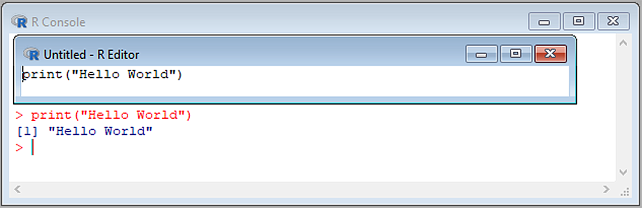
FIGURE 2.5: The R-editor providing code for a famous computational exercise.
There are many other external (to R) IDEs that allow straightforward generation of R script files. Several of these provide a direct link between text editors –that may provide syntax highlighting and auto-completion of R code– and the R-console itself. R IDEs include RWinEdt (an R package plugin for WinEdt ), Tinn-R (a recursive acronym for Tinn is not Notepad), ESS (Emacs Speaks Statistics), Jupyter Notebook (a web-based IDE originally designed for Python, but useful for many languages), and, particularly RStudio, which will be introduced later in this chapter48.
Saved R scripts can be called and executed using the function source(). To browse interactively for source code files, one can type:
or go to File \(>\) Source R code.
2.9 Basic Mathematics
A large number of mathematical operators and functions are available with a conventional download of R. These include mathematical operators, mathematical constants, trigonometric functions, derivative functions, integration approaches, and descriptive statistics functions (Tables 2.3 - 2.9).
2.9.1 Elementary Operations
Elementary mathematical operations and functions (Table 2.3), can be applied to a wide variety of R numeric object classes. For instance, the expression abs(x) could be applied if x was a scalar (e.g., x <- 3), or a collection of numbers, e.g., x <- c(-3, 7, -8). In the latter case, the absolute value would be be calculated for each element in x, and those transformed outcomes would be returned by the function. Notably, this intuitive form of scripting is a dramatic departure from approaches used by many other computer languages49.
| Operation | Function/Operator | To find: | We type: |
|---|---|---|---|
| addition | + |
\(2 + 2\) | 2 + 2 |
| subtraction | - |
\(2 - 2\) | 2 - 2 |
| multiplication | * |
\(2 \times 2\) | 2 * 2 |
| division | / |
\(\frac{2}{3}\) | 2/3 |
| modulo | %% |
remainder of \(\frac{5}{2}\) | 5%%2 |
| integer division | %/% |
\(\frac{5}{2}\) without remainder | 5%/%2 |
| exponentiation | ^ |
\(2^3\) | 2^3 |
| \(\mid x \mid\) | abs(x) |
\(\mid -23.7 \mid\) | abs(-23.7) |
| round \(x\) to \(d\) digits | round(x, digits = d) |
round \(-23.71\) to 1 digit | round(-23.71, 1) |
| round \(x\) up to closest whole num. | ceiling(x) |
ceiling(2.3) | ceiling(2.3) |
| round \(x\) down to closest whole num. | floor(x) |
floor(2.3) | floor(2.3) |
| \(\sqrt{x}\) | sqrt(x) |
\(\sqrt{2}\) | sqrt(2) |
| \(\log_e{x}\) | log(x) |
\(\log_e{5}\) | log(5) |
| \(\log_b{x}\) | log(x, base = b) |
\(\log_{10}{5}\) | log(5, base = 10) |
| \(x!\) | factorial(x) |
\(5!\) | factorial(5) |
| \(\binom{n}{x} = \frac{n!}{x!(n-x)!}\) | choose(n,x) |
\(\binom{5}{2}\) | choose(5,2) |
| \(\Gamma(x)\) | gamma(x) |
\(\Gamma(3.2)\) | gamma(3.2) |
| \(B(a,b) = \frac{\Gamma(a)\Gamma(b)}{\Gamma(a + b)}\) | beta(a,b) |
\(B(3,2)\) | beta(3,2) |
| \(\sum_{i=1}^{n}x_i\) | sum(x) |
sum of x
|
sum(x) |
| cumulative sum | cumsum(x) |
cum. sum of x
|
cumsum(x) |
| \(\prod_{i=1}^{n}x_i\) | prod(x) |
product of x
|
prod(x) |
| cumulative product | cumprod(x) |
cum. prod. of x
|
cumprod(x) |
2.9.2 Associativity and Precedence
Note that the operation:
2 + 6 * 5[1] 32is equivalent to \(2 + (6 \cdot 5) = 32\). This is because the * operator gets higher priority (precedence) than +. Evaluation precedence can be modified with parentheses:
(2 + 6) * 5[1] 40In the absence of operator precedence, mathematical operations in R are (generally) read from left to right (that is, their associativity is from left to right) (Table 2.4). This corresponds to the conventional order of operations in mathematics. For instance:
2 + 2^(2 + 1)[1] 10| Precedent | Operator | Description | Associativity |
|---|---|---|---|
| 1 | ^ |
exponent | right to left |
| 2 | %% |
modulo | left to right |
| 3 |
* /
|
multiplication, division | left to right |
| 4 |
+ -
|
addition, subtraction | left to right |
Example 2.24 \(\text{}\)
Here are some other simple mathematical examples. To solve \(1/\sqrt{22!}\), I could type:
[1] 2.9827e-11And to solve \(\Gamma \left( \sqrt[3]{23\pi} \right)\), I could type:
gamma((23 * pi)^(1/3))[1] 7.411By default the function log() computes natural logarithms, i.e.,
[1] 1The log() function can also compute logarithms to a particular base by specifying the base in an optional second argument called base. For instance, to solve the operation: \(\log_{10}3 + \log_{3}5\), one could type:
[1] 1.9421\(\blacksquare\)
2.9.3 Constants
R allows easy access to most conventional constants (Table 2.5).
| Operation | Operator/Function | To find: | We type: |
|---|---|---|---|
| \(-\infty\) | -Inf |
\(-\infty\) | -Inf |
| \(\infty\) | Inf |
\(\infty\) | Inf |
| \(\pi = 3.141593 \dots\) | pi |
\(\pi\) | pi |
| \(e = 2.718282 \dots\) | exp(1) |
\(e\) | exp(1) |
| \(e^x\) | exp(x) |
\(e^3\) | exp(3) |
2.9.4 Trigonometry
R assumes that the inputs for trigonometric functions (Table 2.6) are in radians. Of course, degrees can be obtained from radians using \(Degrees = Radians \times 180/\pi\), or conversely \(Radians = Degrees \times \pi /180\). Note that there are no base-R functions for cotangent, secant or cosecant. However, for some angle \(x\), measured in radians, these are readily obtained as: \(\cot(x) = \cos(x)/\sin(x)\), \(\sec(x) = 1/\cos(x)\), and \(\csc(x) = 1/\sin(x)\).
| Operation | Operator/Function | To find: | We type: |
|---|---|---|---|
| \(\text{cos}(x)\) | cos(x) |
\(\text{cos}(3 \text{ rad.})\) | cos(3) |
| \(\text{sin}(x)\) | sin(x) |
\(\text{sin}(45^{\circ})\) | sin(45 * pi/180) |
| \(\text{tan}(x)\) | tan(x) |
\(\text{tan}(3 \text{ rad.})\) | tan(3) |
| \(\text{acos}(x)\) | acos(x) |
\(\text{acos}(45^{\circ})\) | acos(45 * pi/180) |
| \(\text{asin}(x)\) | asin(x) |
\(\text{asin}(3 \text{ rad.})\) | asin(3) |
| \(\text{atan}(x)\) | atan(x) |
\(\text{atan}(45^{\circ})\) | atan(45 * pi/180) |
| \(\text{cosh}(x)\) | cosh(x) |
\(\text{cosh}(3 \text{ rad.})\) | cosh(3) |
| \(\text{sinh}(x)\) | sinh(x) |
\(\text{sinh}(45^{\circ})\) | sinh(45 * pi/180) |
| \(\text{tanh}(x)\) | tanh(x) |
\(\text{tanh}(3 \text{ rad.})\) | tanh(3) |
| \(\text{cot}(x)\) | \(\text{cot}(3 \text{ rad.})\) | cos(3)/sin(3) |
|
| \(\text{sec}(x)\) | \(\text{sec}(3 \text{ rad.})\) | 1/cos(3) |
|
| \(\text{csc}(x)\) | \(\text{csc}(3 \text{ rad.})\) | 1/sin(3) |
2.9.5 Derivatives
The function D() finds symbolic and numerical derivatives of simple expressions. It requires two arguments, 1) a mathematical function specified as an object of class expression, and 2) the variable name in the differential (the denominator in the difference quotient).
Objects of class expression, can be created using the function expression(), and evaluated with the function eval()).
Example 2.25 \(\text{}\)
Here is an example of how the functions expression() and eval() can be used:
eval(expression(2 + 2))[1] 4Of course we wouldn’t bother to use expression() and eval() in such simple applications.
\(\blacksquare\)
Table 2.7 contains specific examples using D().
| To find: | We type: |
|---|---|
| \(\frac{d}{dx}5x\) | D(expression(5 * x), "x") |
| \(\frac{d^2}{dx^2} 5x^2\) | D(D(expression(5 * x^2), "x"), "x") |
| \(\frac{\partial}{\partial x} 5xy + y\) | D(expression(5 * x * y + y), "x") |
Example 2.26 \(\text{}\)
Thus, to solve:
\[\frac{d}{dx} 20x^{-4}\]
I could use:
e <- expression(20 * x^(-4))
D(e, "x")
20 * (x^((-4) - 1) * (-4))Unfortunately, it is left to us to simplify the ugly output. That is, \[\begin{aligned} \frac{d}{dx}(20x^{-4}) &= \\ &= 20 \times (x^{(-4 - 1)} \times (-4))\\ &= -80x^{-5} \\ &= -\frac{80}{x^5} \end{aligned}\]
\(\blacksquare\)
Several other R functions provide tidier derivative results compared to D(), although they require the installation and loading of additional packages. See Section 3.10 for a thorough introduction to R packages. For instance, the function Deriv(), from the package Deriv can be applied using two approaches50.
- Under the first approach, a differentiable function is defined as an R
function(see Ch 8) whose one argument is the variable name in the differential. This function is then used as the single required argument inDeriv(). - With the second approach, a differentiable function is defined as a character string. This is then used as the first argument in
Deriv(). The variable name in the differential is defined in a second argument.
Example 2.27 \(\text{}\)
To obtain the derivative in Example 2.26 using Deriv() we would first install the Deriv package (for instance using: install.packages("Deriv")) and load the package using:
library(Deriv) # loads Deriv packageUnder the first approach we could then type:
d <- Deriv(function(x) 20 * x^(-4))
d
function (x)
-(80/x^5)Note that the output, d, is a function, allowing one to obtain instantaneous slopes for specified x values.
d(c(-1, 2, 3, 5.2))[1] 80.000000 -2.500000 -0.329218 -0.021041Under the second approach, we could specify
Deriv("20 * x^(-4)", "x")[1] "-(80/x^5)"Note that the output is a character string.
Both approaches allow one to obtain higher order derivatives and partial derivatives. For instance,
Deriv(d) # second derivativefunction (x)
400/x^6[1] "400/x^6"D() results can also be simplified directly with function Simplify() from the package Deriv. For the current Example, one could use:
e <- expression(20 * x^(-4))
Simplify(D(e, "x"))-(80/x^5)\(\blacksquare\)
2.9.6 Integration
The function integrate solves definite integrals. It requires three arguments. The first is an R function defining the integrand. The second and third are the lower and upper bounds of integration.
Example 2.28 \(\text{}\)
To solve:
\[\int^4_2 3x^2dx\]
we could type:
f <- function(x){3 * x^2}
integrate(f, 2, 4)
56 with absolute error < 6.2e-13\(\blacksquare\)
Note that curly braces, { and }, are used here to define a code block: in this case the body of the function, f. Curly braces can also be used to group programming operations in non-function settings.
Example 2.29 \(\text{}\)
For instance:
{x <- 2
y <- x + 5
y^2
}
[1] 49\(\blacksquare\)
R user-defined functions are explicitly addressed in Ch 8.
2.9.7 Statistics
R, of course, contains a huge number of statistical functions. These will generally require sample data for summarization. Data can be brought into R from spreadsheet files or other data storage files (we will learn how to do this shortly). As we have learned, data can also be assembled in R. For instance,
x <- c(1, 2, 3)Statistical estimators can be separated into point estimators, which estimate an underlying parameter that has a single true value (from a Frequentist viewpoint), and intervallic estimators, which estimate the bounds of an interval that is expected, preceding sampling, to contain a parameter at some probability (Aho 2014). Point estimators can be further classified as estimators of location, scale, shape, and order statistics (Table 2.8). Measures of location estimate the typical or central value from a sample. Examples include the arithmetic mean and the sample median. Measures of scale quantify data variability or dispersion. Examples include the sample standard deviation and the sample interquartile range (IQR). Shape estimators describe the shape (i.e., symmetry and peakedness) of a data distribution. Examples include the sample skewness and sample kurtosis. Finally, the \(k\)th order statistic of a sample is equal to its \(k\)th-smallest value. Examples include the data minimum, the data maximum, and other quantiles (including the median). Intervallic estimators include confidence intervals (Table 2.9). A huge number of other statistical estimating, modelling, and hypothesis testing algorithms are also available for R. For guidance, see Venables and Ripley (2002), Aho (2014), and Fox and Weisberg (2019), among others.
| Acronym | Function | Description | Estimator type |
|---|---|---|---|
| \(\bar{x}\) | mean(x) |
arithmetic mean of \(x\) | location |
mean(x, trim = t) |
trimmed mean of \(x\) for \(0 \leq t \leq 1\). | location | |
| \(GM\) | asbio::G.mean(x) |
geometric mean of \(x\) | location |
| \(HM\) | asbio::H.mean(x) |
harmonic mean of \(x\) | location |
| \(\tilde{x}\) | median(x) |
median of \(x\) | location order statistic |
| \(mode(x)\) | asbio::Mode(x) |
mode of \(x\) | location |
| \(s\) | sd(x) |
standard deviation of \(x\) | scale |
| \(s^2\) | var(x) |
variance of \(x\) | scale |
| \(cov(x,y)\) | cov(x, y) |
covariance of \(x\) and \(y\) | scale |
| \(r_{x,y}\) | cor(x, y) |
Pearson correlation of \(x\) and \(y\) | scale |
| \(IQR\) | IQR(x) |
interquartile range of \(x\) | scale order statistic |
| \(MAD\) | mad(x) |
median absolute deviation of \(x\) | scale |
| \(g_1\) | asbio::skew(x) |
skew of \(x\) | shape |
| \(g_2\) | asbio::kurt(x) |
kurtosis of \(x\) | shape |
| \(min(x)\) | min(x) |
min of \(x\) | order statistic |
| \(max(x)\) | max(x) |
max of \(x\) | order statistic |
| \(\hat{F}^{-1}(p)\) | quantile(x, prob = p) |
quantile of \(x\) at lower-tailed probability \(p\) | order statistic |
| Function | Description |
|---|---|
asbio::ci.mu.z(x, conf, sigma) |
CI for \(\mu\) at level conf. sigma = \(\sigma\). |
asbio::ci.mu.t(x, conf) |
CI for \(\mu\) at level conf. \(\sigma\) unknown. |
asbio::ci.median(x, conf) |
CI for true median at level conf. |
2.10 RStudio
RStudio is an open source IDE for R (Fig 2.6). RStudio greatly facilitates writing R code, saving and examining R objects and history, and many other processes. These include, but are not limited to, tracking and summarizing session workflows and report writing (Section 2.10.2), facilitating R interfaces with other languages and programs (Section 9.1.4), writing R package documentation (Section 10.5), and even developing web-based graphical user interfaces (Section 11.5). RStudio can currently be downloaded at https://posit.co/products/open-source/rstudio/. Like R itself, RStudio can be used with Windows, Mac, and Linux operating systems. Unlike R, RStudio has both freeware and commercial versions51. We will use the former here.

FIGURE 2.6: The RStudio logo.
RStudio is generally implemented using a four pane workspace (Fig 2.7). These panes will contain: 1) the code editor, 2) the R-console, 3) the environment and histories panel, and 4) the plots and other miscellany panel. Tabs in panels will vary depending on the underlying character of the source code being edited, and whether an RStudio project is open (Section 2.10.1).
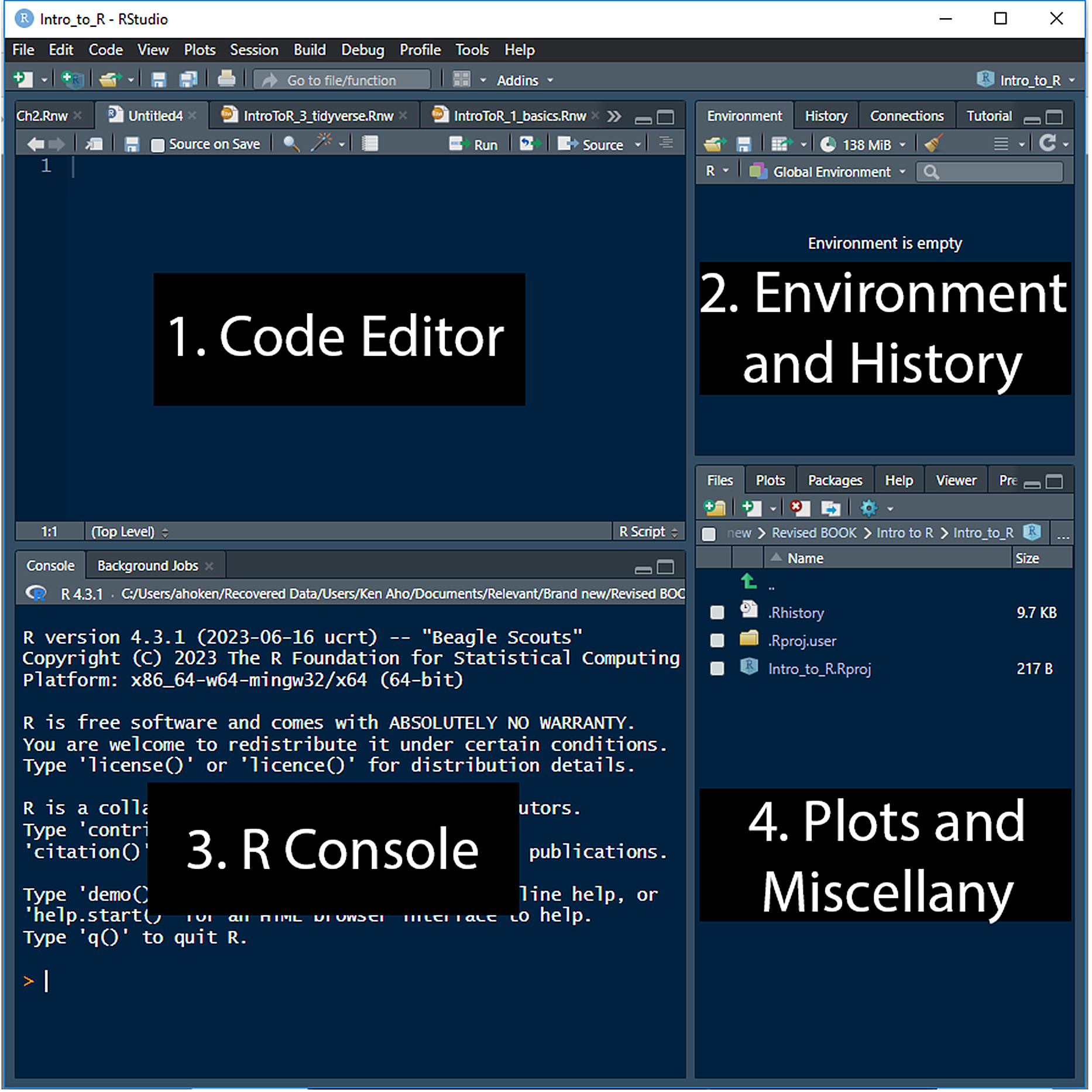
FIGURE 2.7: Interfaces for RStudio (ver 2023.06.2 Build 561).
The RStudio Code Editor panel (Fig 2.7, Panel 1) allows one to create R scripts and even scripts for other languages that can be called to and from R (Ch 9). The code panel can also be used to create and edit session documentation files (see Section 2.10.2 below) and other important R file types. A new R script can be created for editing within the code editor by going to File \(>\) New \(>\) R Script. Commands from an R script can be sent to the R console using the shortcut Ctrl + Enter (Windows and Linux) or Cmd + Enter (Mac).
By default, the R-console panel (Fig 2.7, Panel 2), is identical in functionality to the R console of the most recent version of R on your workstation52. Thus, the console panel can be used to directly enter and execute R code, or to receive commands from the code editor (Panel 1).
The Environments and History panel (Fig 2.7, Panel 3) can be used to: 1) show a list of R objects available in your R session (the Environment tab), or 2) show, search, and select from the history of all previous commands (History tab). This panel also provides an interface for point and click import of data files including .csv, .xls, and many other file formats (Import Dataset pulldown within the Environment tab).
The Plots and Miscellany panel (Fig 2.7, Panel 4) can be used to show: 1) files in the working directory, 2) a scrollable history of plots and image files, and 3) a list of available packages (via the Packages tab), with facilities for updating and installing packages. If a package is in the GUI list, then the package is currently installed. If the package has a check mark next to it, it is loaded. Packages and their installation, updating, and loading are formally introduced in Section 3.10. The panel’s Files pulldown tab allows straightforward establishment of working directories (although this can still be done at the command line using
setwd()) (Fig 2.9). The panel’s Help tap opens automatically when uses?orhelpfor particular R topics (Section 2.5).
CAUTION!
Be very careful when managing files in the Plots and Miscellany panel, as you can permanently delete files without (currently) the possibility of recovery from a Recycling Bin.
2.10.1 RStudio Project
An RStudio project can be be created via the File pulldown menu (Fig 2.9). A project allows all related files (data, figures, summaries, etc.) to be easily organized together by setting the working directory to be the location of the project .Rproj file.
2.10.2 Report Building
One can report analytical workflows and simultaneously run/test R session code in RStudio, using existing markup language systems. Markup languages codify the structure and formatting of a document and the relationships among its components including headings, paragraphs, and hyperlinks (Wikipedia 2025l). In contrast to “what you see is what you get text processing” (reflecting programs like MS Word\(^{\circledR}\)), the term “markup” typically refers to procedural or descriptive languages and processes (including troff, Markdown, HTML, XML, and TeX), in which the final output document may not strongly resemble its underlying source code. In this section I consider two ways to build R reports using this approach.
First, one can create an R Markdown .rmd file that can be compiled to generate an HTML, PDF, or DOC file. Markdown is a highly flexible markup language for creating formatted text using plain-text. R Markdown extends Markdown by allowing users to embed code chunks from R (and other languages) that can be be evaluated and printed during compilation of final output.
Second, one can create a Sweave .rnw file, and use it to compile a PDF document under the TeX document preparation system53. This approach can also be used to print and evaluate code from R and other languages.
The first approach allows a great deal of flexibility in terms of document output (HTML, PDF, and DOC file formats can all be generated from the same R Markdown source file). Further, Markdown is very simple markup language to use, allowing straightforward creation of documents.
The second approach allows full utilization and customization of the TeX system to create beautiful PDF documents (but not other formats). Flexibility in the creation of PDFs is reduced under the first approach because of R Markdown’s reliance on Pandoc to convert from .rmd to .tex markup, see Section 2.10.2.2 below.
It should be emphasized that RStudio is actually not required to build documents from R Markdown .rmd files, or Sweave .rnw files. RStudio simply makes this process easier by providing necessary typesetting systems and packages.
2.10.2.1 Quarto
The Quarto publishing system, released in 2022, is intended to be the “next generation” of R Markdown, and constitutes a third alternative for building reports in RStudio that integrate R, and scripts from other languages. Like R Markdown, Quarto is managed by Posit.
At the surface, Quarto appears very similar to R Markdown. For example, Quarto uses Markdown conventions for creating text, and during knitting in RStudio, a Quarto markup .qmd file will –like an underlying .rmd R Markdown file– be converted to a Markdown .md file before conversion, by Pandoc, into a final document format, e.g., PDF, DOC, HTML (see Section 2.10.2.2 immediately below). However, while R Markdown requires R, Quarto does not. Among other things, this allows straightforward Quarto extendability to the popular Jupyter notebooks IDE. Although, characteristics of the Quarto system are not considered further here, detailed information can be obtained at https://quarto.org/.
2.10.2.2 R Markdown
Steps in R Markdown document processing in RStudio are shown Fig 2.8. These are highly modifiable, but can also be run in a more or less automated manner, requiring little understanding of underlying processes. Use of R Markdown requires the packages rmarkdown (Allaire et al. 2024) and knitr (Xie 2025) which come pre-installed in RStudio.
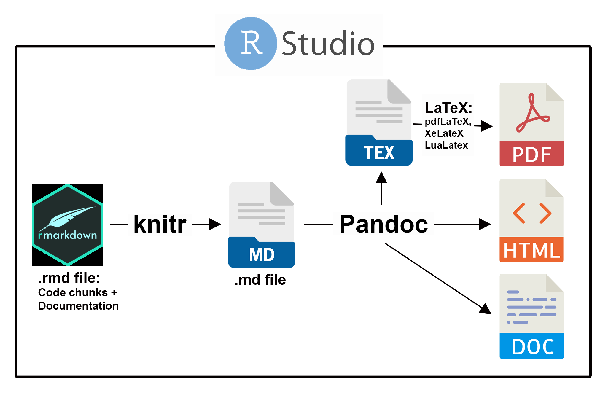
FIGURE 2.8: The process of document creation from an underlying R Markdown (.rmd) file. Functions in the package rmarkdown control conversion of .rmd files to Markdown .md files, using utilities in the package knitr and/or the function Sweave(). Pandoc first creates a .tex file when rendering LaTeX PDF documents.
As an initial step, underlying R Markdown .rmd files (obtainable from RStudio using File > New File > R Markdown) must include a brief YAML54 header (see below) containing document metadata. A summary of YAML features and options in R Markdown is provided in this cheatsheet. R Markdown uses the YAML header to direct Pandoc, a document converter bundled in RStudio, to produce the desired document output55.
The remainder of the .rmd document will contain text written in Markdown syntax, and code chunks which, depending on specified chunk options, will be evaluated and/or printed (see Section 2.10.2.2.2 below). Markdown text, chunks, and their output will be combined into a temporary Markdown .md file which will be converted, by Pandoc, into the desired output format (Fig 2.8). For example, if one has requested HTML output, the simple Markdown text: This is a script will be converted to the HTML formatted: <p>This is a script</p>. One can also write HTML script or CSS code56 directly into an .rmd document (see Section 11.5).
If the desired output is PDF, Pandoc will convert the .md file into a temporary .tex file, which is then processed by the TeX typesetting system to create a PDF file. Support for TeX, and its popular module LaTeX, can be found at a large number of informal user-driven venues, including Stack Exchange and Overleaf, an online LaTeX application57. In Tex typesetting, the tinytex R package (Xie 2024), which installs the stripped-down LaTeX distribution TinyTex, can be used.
Creating an R Markdown document is simple in RStudio. We first open an empty .rmd document by navigating to File \(>\) New File \(>\)R Markdown (Fig 2.9).
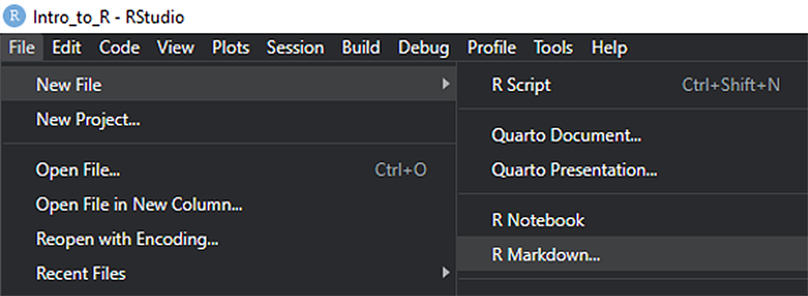
FIGURE 2.9: Part of the RStudio File pulldown menu.
You will delivered to the GUI shown in Fig 2.10. Note that by default Markdown compilation generates an HTML document.
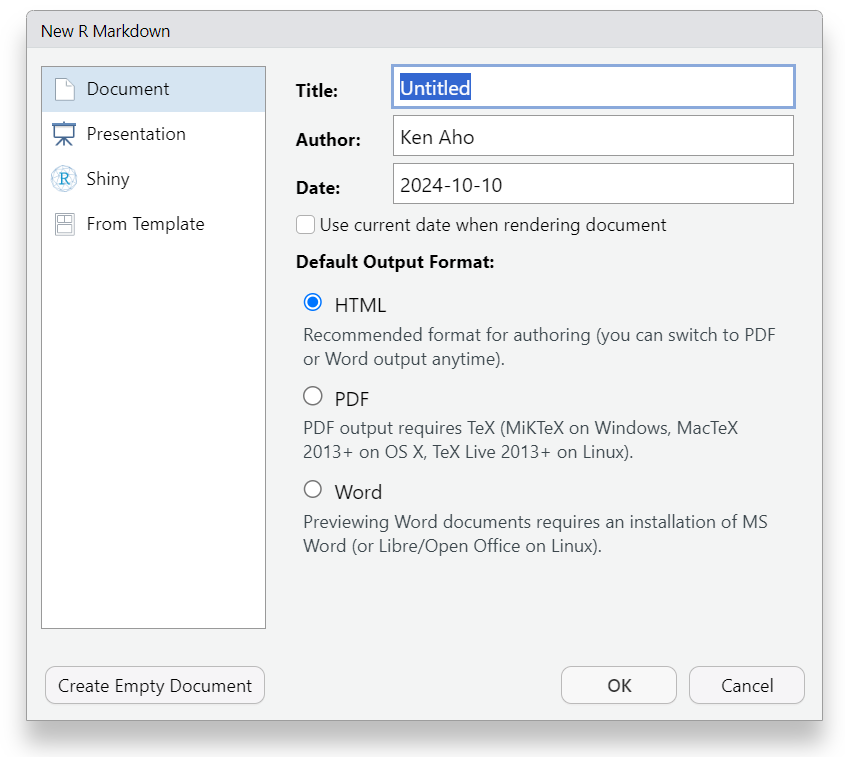
FIGURE 2.10: RStudio GUI for creating an R Markdown document.
The GUI opens an R Markdown (.rmd) skeleton document with a tentative YAML header (Fig 2.11).
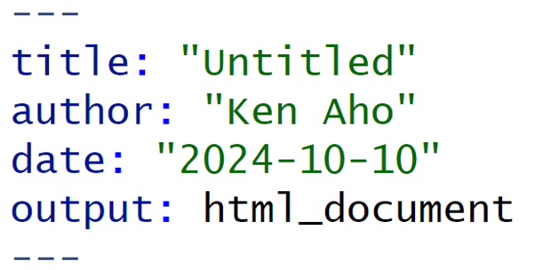
FIGURE 2.11: Simple YAML header for an R Markdown (.rmd) document.
Among other options58, the default HTML output can be changed to one of:
output: pdf_documentto create a LaTeX \(\rightarrow\) PDF document, or
output: word_documentto create a Word\(^{\circledR}\) document.
A potential concern with HTML documents is straightforward portability. Unlike PDF and Word\(^{\circledR}\) documents, HTML files do not internally incorporate images and external library macros. For instance, assume that you generate an HTML from an R Markdown (.rmd) file containing code chunks that produce graphics. These graphics will not be embedded in the HTML file itself. Instead, R Markdown will place them in a folder (named figure) inside the directory containing the HTML output file. When the HTML is opened in a browser program, graphics will be referenced by the HTML and projected into the browser viewer. Thus, if you export an HTML, without its required directory system, it will render incorrectly in a browser. There are currently a number of inexpensive (or free) non-dynamic hosting services, including Amazon Web Services (AWS), GitHub59, and Cloudflare. These can be used to house an HTML (and its required components), allowing it to be rendered correctly when called from a browser.
2.10.2.2.1 Writing Text
Markdown is a relatively simple procedural markup language that allows unformatted text to be written directly into an R Markdown document. There are particular scripting procedures, however, for creating headings, formatted text, and other content.
- Pound signs (e.g.,
#,##,###) can be used as (increasingly nested) hierarchical section delimiters. - Italic, bold, and monospace code fonts can be specified by enclosing text in asterisks, double asterisks, and back ticks, respectively. That is,
*italic*,**bold**, and`code`result in: italic, bold, andcode. - Unordered lists can be created with newlines preceded with asterisks,
*, and ordered lists can be specified with newlines beginning with numbers, e.g.,1.,2., etc. - Superscripts and subscripts can be generated using:
^script^and~script~, respectively. That is,`*r*^2^`and`CO~2~`produce: r2 and CO2. - Footnotes can be created using the format:
`^[footnote]`. - Web hyperlinks can be created using:
`[text](link)`. For instance,`[Amalgam of R](https://www.amalgamofr.org)`creates: Amalgam of R.
By default, RStudio shows R Markdown documents as raw source code. This format, however, can be changed to a more presentational markup (what you see is what you get) format by clicking on the Visual button that appears at the upper left hand side of RStudio Panel 1 (when an R Markdown document is open). The Visual panel contains several interactive menus reminiscent of a word processor (Fig 2.12). These allow users to specify fonts, and to insert LaTeX equations (Section 2.10.2.2.3), section hierarchies, bulleted and numbered lists, and tables.

FIGURE 2.12: Additional RStudio (ver 2026.01.1 Build 403) menu options for an R Markdown document under the Visual viewing mode.
2.10.2.2.2 Writing and Running Code in Chunks
Code from R can be shown, evaluated, and printed on-the fly, within R Markdown documents, by placing code within delineated “chunks”. The can be done using either the knitr package Xie (2015), also installed with RStudio, or with Sweave-style chunks. Switching between these formats in RStudio requires altering options in Build \(>\) Configure Build Tools \(>\) Sweave.
By default, R Markdown will use the knitr R package to print and evaluate code chunks from R –and potentially other programming languages (Section 9.1.4)– into Word, HTML and LaTeX \(\rightarrow\) PDF formats.
One can also use older, Sweave-style, processing of chunks for the same purpose.
Sweave was originally designed to interface with LaTeX, as described in the documentation for the function Sweave() (Leisch 2002). Thus, Sweave provides chunk options to optimize the LaTeX \(\rightarrow\) PDF build process. On the other hand, knitr is intended to support a wide variety of output types (e.g., HTML, PDF (via LaTeX), and Word\(^{\circledR}\)) and provides an extensive set of chunk options to customize input and output, as shown here. Under either approach, R code chunks in R Markdown should begin with ```{r } and end with ```.
In RStudio, code chunks can be inserted into an R Markdown .rnw document by going to Code \(>\) Insert Chunk, or by using the shortcut Ctrl + Alt + I (Windows and Linux) or Cmd + Alt + I (Mac).
Example 2.30 \(\text{}\)
The raw .rnw chunk:
would prompt R Markdown to:
- generate Markdown markup, within the temporary .md document (Fig 2.8), that would show R source code in an appropriate highlighted style, within a rendered document source chunk,
- run the actual R code (i.e., take the mean of the three numbers), and
- render the R evaluation result (print the number
2), by generating appropriate Markdown markup (within the temporary .md document) in a new, potentially distinct, output chunk.
The final result would like this:
[1] 2\(\blacksquare\)
The chunk header, ```{r }, can be used to define additional options. These include the suppression of code evaluation: ```{r , eval = F}, suppression of code printing: ```{r , echo = F}, and/or elimination of the chunk, after running: ```{r , include = F}. For a complete list of chunk options, run
str(knitr::opts_chunk$get())If desired, global options for chunks can be set using an initial R chunk or script (generally with the local chunk option include = F) that defines the components of knitr::opts_chunk.
Example 2.31 \(\text{}\)
For example, to suppress the default insertion of pound signs in lines preceding knitr output (I find this output confusing), throughout the entire knitted document, one could include the initial chunk below.
\(\blacksquare\)
R code can also be invoked inline in a R Markdown document, using the format:
`r some code`For instance, I could seamlessly place three random numbers generated from a the continuous uniform distribution, \(UNIF(0,1)\), inline into text using:
`r runif(3)`Here I run an iteration of the script above using “hidden” inline R code: 0.18281, 0.60523, 0.72919.
2.10.2.2.3 Equations
Inline equations for both R Markdown and Sweave documents (discussed below) can be specified under the LaTeX system, which uses dollar signs, $, to delimit equations. For instance, to obtain the inline equation: \(P(\theta|y) = \frac{P(y|\theta)P(\theta)}{P(y)}\), i.e., Bayes theorem, I could type the LaTeX script into R Markdown:
$P(\theta|y) = \frac{P(y|\theta)P(\theta)}{P(y)}$
Display-style equations can be specified with two dollar signs, $$. For instance, $$P(\theta|y) = \frac{P(y|\theta)P(\theta)}{P(y)}$$ results in:
\[P(\theta|y) = \frac{P(y|\theta)P(\theta)}{P(y)}\]
A cheatsheet for LaTeX equation writing can be found here. A comprehensive list of LaTeX symbols can be found here.
Greater control of equations, and other LaTeX features will be possible in a Sweave .rnw file, compared to an R Markdown .rmd file. This is because .rnw files are converted directly into .tex files (without a Pandoc interface) when building final documents.
2.10.2.2.4 Figures
Probably the simplest way to place external figures into a document is by applying the function knitr::include_graphics() from within a chunk. The following R Markdown code would insert Fig1.jpg (contained in the working directory) into an R Markdown document.
Figures can also be generated from the execution of R plotting functions (see Ch 6, 7). For instance, the following R Markdown code would place a simple R-generated scatterplot into the document:
2.10.2.2.5 Tables
R Markdown tables can be created by specifying the following format (outside of a chunk).
First Header  | Second Header
------------- | -------------
Content Cell  | Content Cell
Content Cell  | Content Cell
Tables, however, can also be be generated by executing R functions within chunks. I generally use the function knitr::kable() to create R Markdown \(\rightarrow\) Pandoc \(\rightarrow\) HTML tables because it is relatively simple to use, and allows straightforward tabling of R output.
Example 2.32 \(\text{}\)
Table 2.10, shows data from the Loblolly dataframe in the package datasets. The data track the growth of loblolly pine trees (Pinus taeda) with respect to seed type and age. The function head(), nested in kable(), allows one to access the first or last components of an R data storage object. Here head() returns the first six dataframe rows.
| height | age | Seed | |
|---|---|---|---|
| 1 | 4.51 | 3 | 301 |
| 15 | 10.89 | 5 | 301 |
| 29 | 28.72 | 10 | 301 |
| 43 | 41.74 | 15 | 301 |
| 57 | 52.70 | 20 | 301 |
| 71 | 60.92 | 25 | 301 |
\(\blacksquare\)
I often use functions in the package xtable to build R Markdown \(\rightarrow\) Pandoc \(\rightarrow\) LaTeX \(\rightarrow\) PDF tables. Under this approach, one could create Table 2.10 using:
This method would also require that one use the command results = 'asis' in the chunk options.
One can even call for different table approaches on the fly. For instance, I could use the command eval = knitr::is_html_output()), in the options of a Markdown chunk when using table code that optimizes HTML formatting, and use eval = knitr::is_latex_output()) to create a table that optimizes LaTeX formatting.
Aside from knitr::kable() and xtable, there are many other R functions and packages that can be used to create R Markdown tables, particularly for HTML output. These include:
- The kableExtra (Zhu et al. 2024) package extends
knitr::kable()by including styles for fonts, features for specific rows, columns, and cells, and straightforward merging and grouping of rows and/or columns. Most kableExtra features extend to both HTML and PDF formats. - DT (Xie et al. 2024), a wrapper for HTML tables that uses the JavaScript (see Section 11.3) library DataTables. Among other features, DT allows straightforward implementation in interactive Shiny apps (Section 11.5).
- Like DT, the reactable package (Lin 2023) creates flexible, interactive HTML embedded tables. As with DT, reactable tables add complications when those interactives are considered as conventional tables in R markdown, with captions and referable labels.
Xie et al. (2020) discuss several other alternatives.
Below I use the function reactable() from the reactable package to create a table with sortable columns and scrollable rows (Table 2.11).
# install.packages("reactable")
library(reactable)
reactable(Loblolly, pagination = FALSE, highlight = TRUE, height = 250)Example 2.33 \(\text{}\)
An R Markdown (.rmd) skeleton file generated by RStudio (Figs 2.9-2.11) contains documentation text, interspersed with example R code in chunks. These been have been modified below to create a simple R markdown document for summarizing the Loblolly dataset (Fig 2.13).
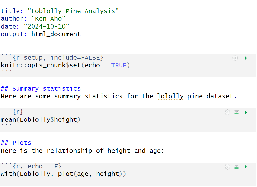
FIGURE 2.13: An R Markdown (.rmd) file with documentation text and interspersed R code in chunks.
Note the use of echo = FALSE in the final chunk to suppress printing of R code. A snapshot of the knitted HTML is shown in Fig 2.14.
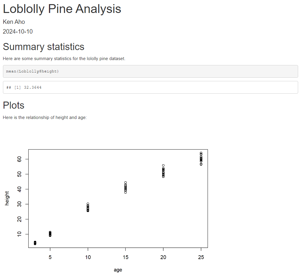
FIGURE 2.14: An HTML document knit from Markdown code in the previous figure. Note that code is displayed (by default) as well as executed.
\(\blacksquare\)
2.10.2.2.6 bookdown
A large number of useful auxiliary features are available for R Markdown, through the R package bookdown (Xie 2023). These include an extended capacity for figure, table, and section numbering and referencing. The bookdown package is not included with RStudio, and will require installation using the code below. See Section 3.10 for more information on loading and installing packages.
install.packages("bookdown") # install bookdown packageTo use bookdown we must modify the output: designation in the YAML header to have a bookdown-specific output. For instance,
output: bookdown::html_document2to create an HTML document, or
output: bookdown::pdf_document2to create a LaTeX \(\rightarrow\) PDF document, or
output: bookdown::word_document2to create an MS Word\(^{\circledR}\) document60.
Numbering R-generated plots and tables in R in bookdown requires specification of a chunk label after the language reference, e.g., r, in the chunk generating the plot or table. Importantly, many table generating R functions (e.g., knitr::kable() and xtable::xtable(), see below) also contain a label argument that allows referencing and numbering.
Example 2.34 \(\text{}\)
In the chunk header below I use the label lobplot. Note that a space is included after r. Captions can be specified in the chunk header using the chunk option fig.cap or tab.cap for figures and tables, respectively. The option fig.cap is used below:
```{r lobplot, echo=FALSE, fig.cap= "Loblolly pine height versus age."}
\(\blacksquare\)
Cross-references within the text can be made using the syntax \@ref(type:label), where label is the chunk label and type is the reference type (e.g., fig, tab, or eq). For Example 2.34, we might want to type something like: “see Figure \@ref(fig:lobplot).” in some non-chunk component of the Markdown document.
Specification of a bookdown output format, will result in automated numbering of sections61. To turn this numbering off, one could modify the YAML output to be:
output:
  bookdown::html_document2:
    number_sections: false
The code indents shown above are important because YAML, like the language Python, uses significant indentation.
To omit numbering for certain sections, one would retain the default bookdown output, and add {-} after the unnumbered section heading, e.g.,
# This section is unnumbered {-}
2.10.2.2.7 Additional Resources for R Markdown and Bookdown
The Posit website houses a number of useful R Markdown guides, including this brief introduction. Thorough descriptions of R Markdown are provided in Xie, Allaire, et al. (2018) and Xie et al. (2020). The latter text is currently available as an online resource. Thorough guidance for bookdown is provided in Xie (2016), which can be viewed as an open-source online document.
2.10.2.3 Sweave
Under the Sweave documentation approach, high quality PDF documents are generated from TeX .tex files, which in turn are created directly from Sweave .rnw files (Fig 2.15). An .rnw document can be considered a .tex document with additional capacities for rendering code chunks and their output (via knitr or Sweave). All non-chunk text in .rnw files, including figure and table captions and cross-referencing must follow Tex (LaTeX) markup syntax and formatting.
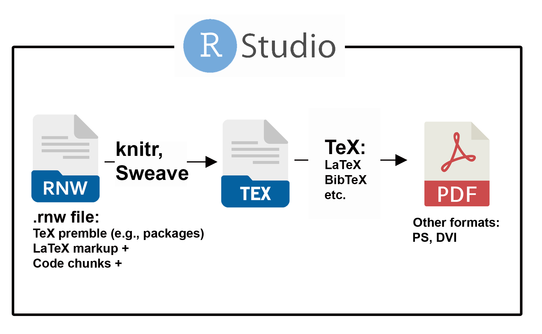
FIGURE 2.15: The process of document creation using an underlying Sweave (.rnw) file. Utilities in the package knitr and/or the function Sweave() control conversion to a .tex file. Conventional TeX processing is then used to create a PDF.
A skeleton .rnw document can be generated in RStudio by going to File \(>\) New File \(>\) R Sweave62.
2.10.2.3.1 Code Chunks in Sweave
Chunks in a Sweave .rnw document can be evaluated using either knitr or Sweave-style approaches (see Section 2.10.2.2.2). As before, switching between these formats in RStudio requires altering options in Build \(>\) Configure Build Tools \(>\) Sweave. In .rnw documents, code chunks are initiated which <<>>=, which serves as a chunk header, and are closed with @.
Example 2.35 \(\text{}\)
Including the chunk below in an .rnw file would: 1) cause the R source code to be printed in a LaTeX-rendered PDF, 2) run the code in R (the mean of the three number would be calculated), and 3) print the evaluated result in the output PDF.
\(\blacksquare\)
Chunk options in Sweave are generally similar to those in knitr, but are more limited (see vignette("Sweave")).
Example 2.36 \(\text{}\)
In Fig 2.16 I create an .rnw file, based on an RStudio skeleton, with text and analyses reflecting those used with R Markdown in Example 2.33. We note that instead of the Markdown YAML header, we now have conventional TeX lines in the preamble defining the type of desired document (e.g., article) and the packages needed for document compilation (e.g., amsmath). The authoritative source for TeX/LaTeX packages and related materials is CTAN (Comprehensive TeX Archive Network)63. Tex packages can be downloaded from CTAN using open source TeX distribution software, including MikTeX and Tex Live.
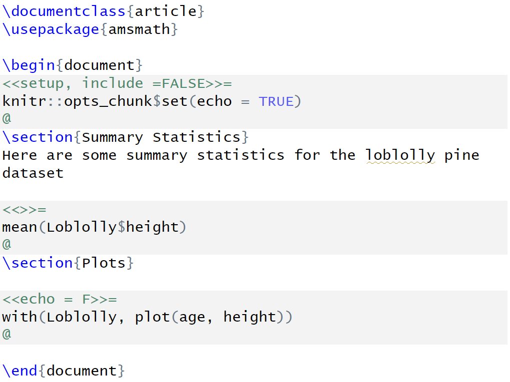
FIGURE 2.16: A Sweave (.rnw) file with documentation text and interspersed code in chunks.
Fig 2.17 shows a snapshot of the result, following automated .rnw \(\rightarrow\) knitr \(\rightarrow\) LaTeX \(\rightarrow\) .pdf compilation in RStudio.
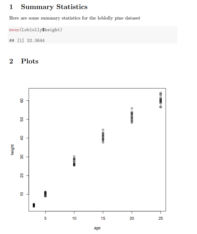
FIGURE 2.17: A .pdf document resulting from compilation of Sweave code in the previous figure.
\(\blacksquare\)
2.10.2.4 Purl
R chunk code can be extracted from an .rmd or an .rnw file using the function knitr::purl(). For instance, assume that the R Markdown loblolly pine summary shown in Fig 2.13 is saved in the working directory under the name lob.rmd. Code from the file will be extracted to a script file called lob.R, located in the working directory, if one types:
purl("lob.rmd")Exercises
-
Create an R Markdown document to contain your homework assignment. Modify the YAML header to allow numbering of figures and tables, but not sections. This will require use of the bookdown package (see Section 2.10.2.2.6). Install bookdown at the R console (not within a document chunk). To test the formatting, perform the following steps:
- Create a section header called
Question 1and a subsection header called (a). Under (a) type"completed". - Under the subsection header (b), insert a chunk, and create a simple plot of points at the coordinates: \(\{1,1\}\), \(\{2,2\}\), \(\{3,3\}\), by typing the code:
plot(1:3)in the chunk. Create a label for the chunk, and a create caption for the plot using the knitr chunk option,fig.cap(see Example 2.34). - Under the subsection header (c), create a cross reference for the plot from (b) (see Section 2.10.2.2.6).
- Under the subsection header (d), write the equation, \(y_i = \hat{\beta}_0 + \hat{\beta}_1x_i + \hat{\varepsilon_i}\), using LaTeX. As noted earlier, a LaTeX equation cheatsheet can be found here.
- Render (knit) the final document as either an .html file or a .doc file. Include other assigned exercises for this Chapter as directed, using the general formatting approach given in Question 1.
- Create a section header called
-
Perform the following operations.
- Leave a note to yourself.
- Create and examine an object called
xthat contains the numeric entries 1, 2, and 3. - Make a copy of
xcalledy. - Show the class of
y. - Show the base type of
y. - Show the attributes of
y. - List the current objects in your work session.
- Identify your working directory.
Distinguish R expressions and assignments.
-
Sometimes R reports unexpected results for its classes and base types.
- Create
x <- factor("a","a","b")and show the class ofx. - Type
?factor. What is afactorin R? - Show the base type of
x? Is this surprising? Why? Type?integer. What is anintegerin R?
- Create
-
\(\bigstar\) With respect to R OOP characteristics:
- What are R OO and base objects, and do both have explicit class attributes?
- What are implicit and explicit classes in R, and how can you identify them?
\(\bigstar\) Create a custom
.Rprofilefile located in R_USER or the current working directory (or modifyRprofile.sitein R_HOME/etc) so that R welcomes you during start-up.-
Solve the following mathematical operations using R.
- \(1 + 3/10 + 2\)
- \((1 + 3)/10 + 2\)
- \(\left(4 \cdot \frac{(3 - 4)}{23}\right)^2\)
- \(\log_2(3^{1/2})\)
- \(3\boldsymbol{x}^3 + 3\boldsymbol{x}^2 + 2\) where \(\boldsymbol{x} = \{0, 1.5, 4, 6, 8, 10\}\)
- \(4(\boldsymbol{x} + \boldsymbol{y})\) where \(\boldsymbol{x} = \{0, 1.5, 4, 6, 8\}\) and \(\boldsymbol{y} = \{-2, 0.5, 3, 5, 8\}\).
- \(\frac{d}{dx} \tan(x) 2.3 \cdot e^{3x}\)
- \(\frac{d^2}{dx^2} \frac{3}{4x^4}\)
- \(\int_3^{12} 24x + \ln(x)dx\)
- \(\int_{-\infty}^{\infty} \frac{1}{\sqrt{2\pi}}e^{-\frac{x^2}{2}}dx\) (i.e., find the area under a standard normal pdf).
- \(\int_{-\infty}^{\infty}\frac{x}{\sqrt{2\pi}}e^{-\frac{x^2}{2}}dx\) (i.e., find \(E(X)\) for a standard normal pdf).
- \(\int_{-\infty}^{\infty}\frac{x^2}{\sqrt{2\pi}}e^{-\frac{x^2}{2}}dx\) (i.e., find \(E(X^2)\) for a standard normal pdf).
- Find the sum, cumulative sum, product, cumulative product, arithmetic mean, median and variance of the data
x = c(0, 1.5, 4, 6, 8, 10).
The velocity of the earth’s rotation on its axis at the equator, \(E\), is approximately 1674.364 km/h, or 1040.401 m/h64. We can calculate the velocity of the rotation of the earth at any latitude with the equation, \(V = \cos(\)latitude\(^\text{o}) \times E\). Using R, simultaneously calculate rotational velocities for latitudes of 0,30,60, and 90 degrees north, or south, latitude (they will be the same). Remember, the function
cos()assumes inputs are in radians, not degrees.