5 Welcome to the Tidyverse

“There’s more than one way to do it.”

- Larry Wall, creator of the Perl programming language

5.1 The Tidyverse

This chapter demonstrates the data management capabilities of the tidyverse (Wickham et al. 2019). Thus, Chapter 5 can be considered a tidyverse reconsideration of Ch 4. The tidyverse is currently a collection of nine core packages (Fig 5.1). These are:

dplyr Grammar and functions for data manipulation.
forcats Tools for solving common problems with factors.
ggplot2 A system for “declaratively creating graphics”, based on the book The Grammar of Graphics (Wilkinson 2012).
purrr An enhancement of R’s functional programming (FP) toolkit.
readr Methods for reading rectangular data.
stringr Functions to facilitate working with strings.
tibble A “modern re-imagining of the data frame.”
tidyr A set of functions for “tidying data.”
lubridate Applications for date-time data.

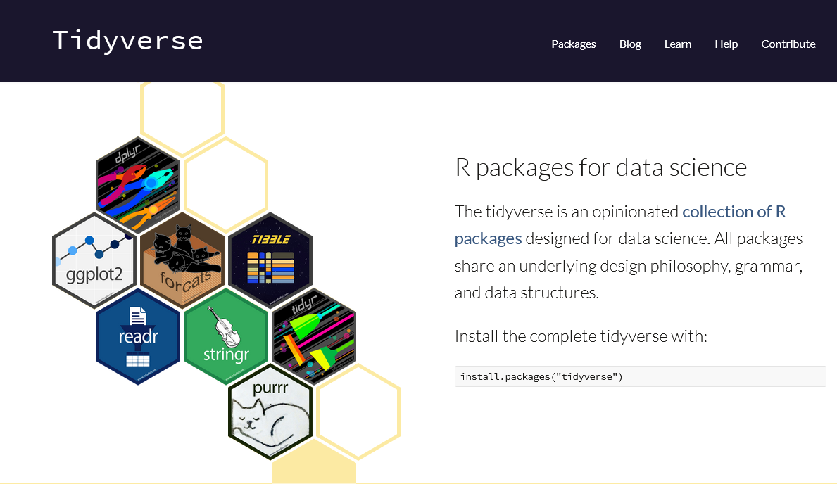
FIGURE 5.1: The main packages of the tidyverse.

The tidyverse library also contains several useful ancillary packages, including reshape2, hms, blob, margrittr, and glue. While installing tidyverse will result in the installation of both main and ancillary packages, loading the tidyverse will result only in the complete loading of the eight main tidyverse packages.

Importantly, this chapter is not meant to be an authoritative summary of the tidyverse. Coverage here is mostly limited to the core data management packages magrittr, tibble, dplyr, stringer, and lubridate and the ancillary package and reshape2. The tidyverse ggplot2 package is the major focus of Chapter 7. Wickham et al. (2023) provides a succinct but thorough introduction to the tidyverse in the open source book R for Data Science. Useful tidyverse “cheatsheets” can be found here.

The tidyverse packages can be downloaded using:

install.packages("tidyverse")

5.2 Pipes

The tidyverse frequently uses pipe operators. In programming, a pipe is a set of commands connected in series, wherein the output of one command is the input of the next⁹². In many cases, use of pipes allows clearer representations of coding processes⁹³. Pipe processes are often described using familial terms to represent their hierarchy and relationships:

\[\begin{equation} \text{parent process} \Rightarrow \text{child process} \Rightarrow \text{grandchild process} \tag{5.1} \end{equation}\]

where $\Rightarrow$ represents a pipe.

As of R 4.1, the preferred pipe operator for the tidyverse is the forward pipe, |>. The |> pipe, which is housed in the base package, was motivated by an older pipe operator from the tidyverse package magrittr, %>%. The %>% pipe, which generally performs identically to |>, can still be used if magrittr is loaded⁹⁴.

Example 5.1 $\text{}$
Consider the circular operation: $\log_e(\exp(1))$. We could write this as,

1 |> exp() |> log()

[1] 1

Here the number $1$ is piped into the function exp(), with the result: $\exp(1) = e^1 = e$, and this outcome is piped into the function log(), with the result: $\log_e e = 1$. Because the first arguments of exp() and log() are simply calls to numeric data, and these are provided by the previous pipe segment, we do not have to include information about x for f(x) operations. Thus, when functions require only the previous pipe segment result as an argument, then x |> f() is equivalent to $f(x)$. In the case that multiple arguments need to be specified, the script x |> f(y) is equivalent to $f(x, y)$,

2 |> log(base = 2)

[1] 1

and x |> f(y) |> g(z) describes $g(f(x, y), z)$,

2 |> log(base = 2) |> exp()

[1] 2.7183

$\blacksquare$

Example 5.2 $\text{}$
This example illustrates that the forward pipe works recursively from the result of the previous pipe segment, using the loblolly pine dataset.

head(Loblolly) # First 6 rows of data

Grouped Data: height ~ age | Seed
   height age Seed
1    4.51   3  301
15  10.89   5  301
29  28.72  10  301
43  41.74  15  301
57  52.70  20  301
71  60.92  25  301

Loblolly |>
head() |>
tail(2) # Last 2 rows from first 6 rows

Grouped Data: height ~ age | Seed
   height age Seed
57  52.70  20  301
71  60.92  25  301

$\blacksquare$

Example 5.3 $\text{}$
We can define the result of a pipe to be an object in the current environment (Sections 2.4.5, 8.2). Consider the script and output below (Fig 5.2).

x <- seq(1,10,length=100)
y <- x |> sin() # result of pipe is object y
plot(x, y, type = "l", ylab = "sin(x)", xlab = "x (radians)")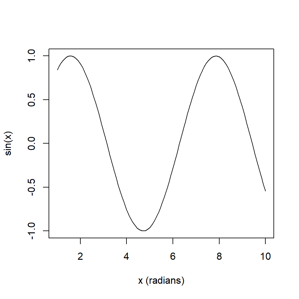

FIGURE 5.2: Creating a global variable (object) resulting from a pipeline.

We will formally consider the function plot() in Ch 6.

$\blacksquare$

5.2.1 Other pipes

The operator |> is more syntactically (and algorithmically) streamlined than %>%. However, there are several features available to %>% that do not exist for |>. These include the dot placeholder operator, ., which allows operations like $f(x,y)$ by specifying x %>% f(.,y). The %>% forward pipe does not even require the argument-less “use defaults” designation, (). That is, $f(x)$ can be expressed as x %>% f.

Example 5.4 $\text{}$

Here I use the dot placeholder, ..

library(magrittr)


Attaching package: 'magrittr'

The following object is masked from 'package:rlang':

    set_names

2 %>% log(., base = .)

[1] 1

To accomplish this operation with |>, I would have to create a function (Ch 8), place it in parentheses, and then call it:

2 |> (function(b){log(b, base = b)})()

[1] 1

Here I call log(), without using ().

exp(1) %>% log

[1] 1

$\blacksquare$

It is worth noting that, in addition to %>%, magrittr contains several other useful pipe operators. These include the assignment pipe and the tee pipe. The assignment pipe operator, %<>%, will pipe x into one or more f(x) expressions, and then assign the result to the name x⁹⁵. The tee pipe operator %T>% works like %>%, except the return value in x %T>% f(x) is x itself. This is useful when a pipeline requires a side-effect like plotting or printing⁹⁶. Despite these potential benefits, we follow Wickham et al. (2023), and focus on |> not magrittr pipes, here.

5.3 tibble

The tidyverse package tibble provides an alternative to the data.frame format of data storage, called a tibble. Tibbles have classes dataframe and tbl_df, allowing them to posses additional characteristics including enhanced printing (see Example 5.5 below). Additional distinguishing characteristics of tibbles include: 1) a character vector is not automatically coerced to have class factor, 2) recycling (see Section 3.1.1) only occurs for an input of length one, and 3) there is no partial matching when $ is used to index by tibble columns by name⁹⁷. The functions tibble() generates tibbles. The function as_tibble() coerces a dataframe to be a tibble.

Example 5.5 $\text{}$
Here we compare dataframe and tibble output of the same data.

data <- data.frame(numbers = 1:3, letters = c("a","b","c"),
                   date = as.Date(c("2021-12-1", "2021-12-2",
                                    "2021-12-2"),
                           format = "%Y-%m-%d"))
data

  numbers letters       date
1       1       a 2021-12-01
2       2       b 2021-12-02
3       3       c 2021-12-02

library(tidyverse)
datat <- as_tibble(data)
datat

# A tibble: 3 × 3
  numbers letters date      
    <int> <chr>   <date>    
1       1 a       2021-12-01
2       2 b       2021-12-02
3       3 c       2021-12-02

$\blacksquare$

5.4 dplyr

The dplyr package contains a collection of core tidyverse algorithms for data summarization and manipulation⁹⁸. Table 5.1 lists some useful dplyr functions.

Function	Use	Intent
`filter()`	Subset rows using logical expressions.	R
`arrange()`	Reorder rows of a dataframe.	R
`mutate()`	New columns from functions of existing data.	C
`across()`	Transform or summarize multiple columns.	C
`select()`	Select dataframe columns.	C
`rename()`	Rename dataframe columns.	C
`summarize()`	Summarize dataframe columns, allows groups.	G
`group_by`	Group dataframe using categories.	G
`slice_`	Extract dataframe rows by group.	G

5.4.1 `filter()`

The function filter() provides a straightforward way to extract dataframe rows based on Boolean operators.

Example 5.6 $\text{}$
Here we obtain rows in Loblolly associated with seed type 301.

Loblolly |>
  filter(Seed == "301")

Grouped Data: height ~ age | Seed
   height age Seed
1    4.51   3  301
15  10.89   5  301
29  28.72  10  301
43  41.74  15  301
57  52.70  20  301
71  60.92  25  301

Here are Loblolly rows associated with height responses greater than 60 feet.

Loblolly |>
  filter(height > 60)

Grouped Data: height ~ age | Seed
   height age Seed
71  60.92  25  301
72  63.39  25  303
73  64.10  25  305
75  63.05  25  309
77  60.07  25  315
78  60.69  25  319
79  60.28  25  321
80  61.62  25  323

$\blacksquare$

5.4.2 `arrange()`

The function arrange() orders the rows of a data frame based on the alphanumeric ordering of specified data.

Example 5.7 $\text{}$
Here we use arrange() to sort the result from the previous Example (Ex 5.7) from smallest to largest loblolly pine heights.

Loblolly |>
  filter(height > 60) |>
  arrange(height)

Grouped Data: height ~ age | Seed
   height age Seed
77  60.07  25  315
79  60.28  25  321
78  60.69  25  319
71  60.92  25  301
80  61.62  25  323
75  63.05  25  309
72  63.39  25  303
73  64.10  25  305

One can use arrange(desc()) to sort a dataframe in descending (largest-to-smallest) order.

Loblolly |>
  filter(height > 60) |>
  arrange(desc(height))

Grouped Data: height ~ age | Seed
   height age Seed
73  64.10  25  305
72  63.39  25  303
75  63.05  25  309
80  61.62  25  323
71  60.92  25  301
78  60.69  25  319
79  60.28  25  321
77  60.07  25  315

$\blacksquare$

5.4.3 `mutate()`

The function mutate() creates new dataframe columns that are functions of existing variables.

Example 5.8 $\text{}$
Below I rename the column height, height.ft, using the function dplyr::rename(), and create a new column of height in meters using mutate().

Loblolly |>
  rename(height.ft = height) |>
  mutate(height.m = height.ft * 0.3048) |>
  head(3)

$\blacksquare$

5.4.4 `select()`

The select() function allows one to select particular columns in a data frame.

Example 5.9 $\text{}$
For instance, here I select height from Loblolly.

Loblolly |>
  select(height) |>
  head()

$\blacksquare$

The select() function can be used in more sophisticated ways by combining it with other dplyr functions like starts_with() and ends_with(), or other Boolean operators.

Example 5.10 $\text{}$
He we select the height and age columns by calling for variable names that start with "h" or end with "e".

Loblolly |>
  select(starts_with("h"), ends_with("e")) |>
  head(3)

   height age
1    4.51   3
15  10.89   5
29  28.72  10

$\blacksquare$

5.4.5 `summarize()`

The function summarize(), or equivalently summarise(), creates a new data frame with one row for each combination of specified grouping variables. If no groups are given (for instance, in the case that group_by is not used to group data, Section @ref(tidy_groupby) below), dataframe rows will be summaries of all observations in the required input .data argument (which can be piped in).

Example 5.11 $\text{}$
Here we use summarize() to obtain means for loblolly pine height (in feet) and age (in years).

Loblolly |>
  summarise(mean.height.ft = mean(height), mean.age.yrs = mean(age))

  mean.height.ft mean.age.yrs
1         32.364           13

$\blacksquare$

5.4.6 `across()`

The dplyr function across() allows one to apply the same transformation to multiple columns. Specifying the first argument in across() as everything() would allow application of a function or transformation to all columns in a dataframe.

Example 5.12 $\text{}$
Here we center (subtract the mean) from the age and height columns in Loblolly using across() and mutate().

Loblolly |>
   mutate(across(c(age, height), function(x)x-mean(x))) |>
  head(3)

Grouped Data: height ~ age | Seed
     height age Seed
1  -27.8544 -10  301
15 -21.4744  -8  301
29  -3.6444  -3  301

$\blacksquare$

Conjoining across() and summarize() provides a tidyverse equivalent of apply(X, MARGIN = 2, FUN)

Example 5.13 $\text{}$
Here I take the median of the age and height columns.

Loblolly |>
   summarize(across(c(age, height), median))

   age height
1 12.5     34

$\blacksquare$

5.4.7 `group_by()`

The group_by() function is often used in conjunction with other dplyr functions, including summarize(), to provide an underlying grouping framework for data summaries.

Example 5.14 $\text{}$
Here we use group_by() with summarize() to describe the Loblolly height data. Specifically, we will take the mean and the variance of Loblolly$height with respect to categories specified in group_by().

Loblolly |>
  group_by(Seed) |>
  summarise(mean.height.ft = mean(height),
            var.height.ft2 = var(height)
            ) |>
  head(5)

# A tibble: 5 × 3
  Seed  mean.height.ft var.height.ft2
  <ord>          <dbl>          <dbl>
1 329             30.3           443.
2 327             30.6           440.
3 325             31.9           468.
4 307             31.3           494.
5 331             31.0           495.

More than one grouping variable can be specified in group_by():

Loblolly |>
  group_by(Seed, age) |>
  summarise(mean.height.ft = mean(height),
            var.height.ft2 = var(height)
            ) |>
  head(5)

# A tibble: 5 × 4
  Seed    age mean.height.ft var.height.ft2
  <ord> <dbl>          <dbl>          <dbl>
1 329       3           3.93             NA
2 329       5           9.34             NA
3 329      10          26.1              NA
4 329      15          37.8              NA
5 329      20          48.3              NA

Clearly, group_by() and summarise() allow more options than the base function tapply() (Section 4.1.1.4). The latter function only provides summaries of groups within a single categorical INDEX, with respect to a single quantitative vector, and a single user-defined function.

Starting with dplyr 1.1.0, we can use the .by argument in summarize to bypass group_by(), although this argument is experimental, and may be deprecated in the future (see ?summarise).

Loblolly |>
  summarise(mean.height.ft = mean(height),
            var.height.ft2 = var(height),
            .by = Seed) |>
  head(5)

  Seed mean.height.ft var.height.ft2
1  301         33.247         512.50
2  303         34.107         552.24
3  305         35.115         572.51
4  307         31.328         493.83
5  309         33.782         535.12

$\blacksquare$

5.4.8 The `slice_` functions

The helpful slice_ functions allow subsetting of the rows of a dataframe using various criteria. Assume we have dataframe df with r rows.

df |> slice_head(n = x) gives rows 1:x.
df |> slice_tail(n = x) gives rows (r-x):r.
df |> slice_min(y, n = x) gives the row(s) with x smallest value(s) of column y.
df |> slice_max(y, n = x) gives the row(s) with x largest value(s) of column y.
df |> slice_sample(x, n = x) extracts x random rows.

When used with group_by, the functions perform the specified operations for each group.

Example 5.15 $\text{}$
Consider:

Loblolly |>
  slice_head(n = 2)

Grouped Data: height ~ age | Seed
   height age Seed
1    4.51   3  301
15  10.89   5  301

Loblolly |>
  slice_min(height, n = 2)

Grouped Data: height ~ age | Seed
   height age Seed
14   3.46   3  331
9    3.77   3  321

Loblolly |>
  group_by(Seed) |>
  slice_max(height, n = 2) |>
  head(4)

# A tibble: 4 × 3
# Groups:   Seed [2]
  height   age Seed 
   <dbl> <dbl> <ord>
1   56.4    25 329  
2   48.3    20 329  
3   56.8    25 327  
4   48.4    20 327

$\blacksquare$

5.5 stringr

As evident in Section 4.3, use of regular expressions for matching, querying and substituting strings can be confusing. The stringr package attempts to simplify some of these difficulties. The stringr package uses processing tools from the package stringi (Gagolewski 2022) for pattern searching under a wide array of potential approaches. All stringr functions have the prefix str_ and take a character string or string vector as the first argument.

Consider the vector of plant scientific names used to demonstrate string management in Section 4.3.

names = c("Achillea millefolium", "Aster foliaceus",
                           "Elymus scribneri", "Erigeron rydbergii",
                           "Carex elynoides", "Carex paysonis",
                           "Taraxacum ceratophorum")

Example 5.16 $\text{}$
The function str_length() can be used to count the number of characters in a string.

str_length(names)

[1] 20 15 16 18 15 14 22

$\blacksquare$

Example 5.17 $\text{}$
The function str_detect() tests for the presence or absence of a pattern in a string. Here I test for "Aster" (the genus Aster).

str_detect(names, "Aster")

[1] FALSE  TRUE FALSE FALSE FALSE FALSE FALSE

Here are entries not containing Aster.

str_detect(names, "Aster", negate = TRUE)

[1]  TRUE FALSE  TRUE  TRUE  TRUE  TRUE  TRUE

$\blacksquare$

Example 5.18 $\text{}$
Here we subset names using the function stringr::str_subset() to obtain species within the genus Carex.

str_subset(names, "Carex")

[1] "Carex elynoides" "Carex paysonis"

$\blacksquare$

Example 5.19 $\text{}$
The function str_replace() is analogous to the base R function gsub(). It can be used to replace text based on a pattern.

str_replace(names, "Carex", "C.")

[1] "Achillea millefolium"   "Aster foliaceus"       
[3] "Elymus scribneri"       "Erigeron rydbergii"    
[5] "C. elynoides"           "C. paysonis"           
[7] "Taraxacum ceratophorum"

$\blacksquare$

Most stringr functions work with regular expressions (Section 4.4).

Example 5.20 $\text{}$
Here we count upper and lower case vowels with the function stringr::str_count() using a pattern defined by the regex character class [AEIOUaeiou].

str_count(names, "[AEIOUaeiou]")

[1] 9 7 5 7 6 5 9

and use stringr::str_extract() to extract strings nine alphanumeric characters long, and then sort the strings with a pipe.

str_extract(names, "[[:alnum:]]{9}") |>
  sort()

[1] "elynoides" "foliaceus" "millefoli" "rydbergii" "scribneri" "Taraxacum"

$\blacksquare$

5.6 lubridate

Base R approaches for handling date-time data are described in Section 4.5. The package lubridate (https://lubridate.tidyverse.org/) contains functions for simplifying and extending some of these operations.

Example 5.21 $\text{}$
As an example dataset, I will use the time series used to illustrate date-time classes in Section 4.5.

dates <- c("08/13/2019 04:00", "08/13/2019 06:30", "08/13/2019 09:00",
           "08/13/2019 11:30", "08/13/2019 14:00", "08/13/2019 16:30",
           "08/13/2019 19:00", "08/13/2019 21:30", "08/14/2019 00:00",
           "08/14/2019 02:30", "08/14/2019 05:00", "08/14/2019 07:30",
           "08/14/2019 10:00", "08/14/2019 12:30", "08/14/2019 15:00",
           "08/14/2019 17:30", "08/14/2019 20:00", "08/14/2019 22:30",
           "08/15/2019 01:00", "08/15/2019 03:30")

library(lubridate)

We will define the timezone to be timezone of our computer workstation.

tz <- Sys.timezone(location = TRUE)

The package lubridate contains data-time parsers that may be easier to use than the base functions strptime and as.Date. For the current example, we note that the data are in a month/day/year hour:minute format. So we can create a time series using the function lubridate::mdy_hm.

date_lub <- mdy_hm(dates, tz = tz)
date_lub

 [1] "2019-08-13 04:00:00 MDT" "2019-08-13 06:30:00 MDT"
 [3] "2019-08-13 09:00:00 MDT" "2019-08-13 11:30:00 MDT"
 [5] "2019-08-13 14:00:00 MDT" "2019-08-13 16:30:00 MDT"
 [7] "2019-08-13 19:00:00 MDT" "2019-08-13 21:30:00 MDT"
 [9] "2019-08-14 00:00:00 MDT" "2019-08-14 02:30:00 MDT"
[11] "2019-08-14 05:00:00 MDT" "2019-08-14 07:30:00 MDT"
[13] "2019-08-14 10:00:00 MDT" "2019-08-14 12:30:00 MDT"
[15] "2019-08-14 15:00:00 MDT" "2019-08-14 17:30:00 MDT"
[17] "2019-08-14 20:00:00 MDT" "2019-08-14 22:30:00 MDT"
[19] "2019-08-15 01:00:00 MDT" "2019-08-15 03:30:00 MDT"

Other lubridate parsers include ymd(), ymd_hms(), dmy(), dmy_hms(), and mdy(). The lubridate parsers can often handle mixed methods of data entry. From the ymd() documentation we have the following example:

x <- c(20090101, "2009-01-02", "2009 01 03", "2009-1-4",
       "2009-1, 5", "Created on 2009 1 6", "200901 !!! 07")
ymd(x)

[1] "2009-01-01" "2009-01-02" "2009-01-03" "2009-01-04" "2009-01-05"
[6] "2009-01-06" "2009-01-07"

$\blacksquare$

Lubridate also allows extended mathematical operations for its date-time objects with the functions duration(), period(), and interval().

Example 5.22 $\text{}$
Duration functions include dseconds(), dminutes(), ddays(), and dmonths().

duration("12m", units = "seconds") # seconds in 1 year

[1] "31557600s (~1 years)"

dmonths(12)

[1] "31557600s (~1 years)"

date_lub[1]

[1] "2019-08-13 04:00:00 MDT"

date_lub[1] + ddays(1)

[1] "2019-08-14 04:00:00 MDT"

$\blacksquare$

Example 5.23 $\text{}$
Periodic functions include seconds(), minutes(), hours(), and days().

days(12) + minutes(2) + seconds(3)

[1] "12d 0H 2M 3S"

date_lub[1]

[1] "2019-08-13 04:00:00 MDT"

date_lub[1] - days(12)

[1] "2019-08-01 04:00:00 MDT"

$\blacksquare$

Example 5.24 $\text{}$
Interval functions include int_length(), int_start(), and int_end().

int <- interval(start = first(date_lub), end = last(date_lub))

int_length(int) |>
  duration()

[1] "171000s (~1.98 days)"

$\blacksquare$

5.7 reshape2

Tidyverse functions generally require that data are in a long table format. That is, data are stored with columns containing all the values for a particular variable of interest. Unfortunately, this format is not conventional for many scientific applications, particularly longitudinal studies that follow experimental units over time. These will often have a wide table format. The tidyverse reshape2 package contains several functions for converting dataframes from wide to a long table formats, including the functions reshape2::melt() and tidyr::gather(). The reshape2::melt.data.frame() function generates a value column based on data commonalities of outcomes given in a variable or variables defined in the id argument. A remaining column, if any, that captures these commonalities will be given the name variable. The names of the value and variable output columns can be changed with the arguments value.name and variable.name, respectively.

Example 5.25 $\text{}$
Consider the asbio::asthma dataset, which has a wide table format. The dataset documents the effect of three respiratory treatments (measured as Forced Expiratory Volume in one second (FEV1)) for 24 asthmatic patients over time (11H - 18H, i.e, hour 11 to hour 18). A baseline measure of FEV1 (BASEFEV1) was also taken 11 hours before application of the treatment.

data(asthma)
head(asthma)

  PATIENT BASEFEV1 FEV11H FEV12H FEV13H FEV14H FEV15H FEV16H FEV17H FEV18H
1     201     2.46   2.68   2.76   2.50   2.30   2.14   2.40   2.33   2.20
2     202     3.50   3.95   3.65   2.93   2.53   3.04   3.37   3.14   2.62
3     203     1.96   2.28   2.34   2.29   2.43   2.06   2.18   2.28   2.29
4     204     3.44   4.08   3.87   3.79   3.30   3.80   3.24   2.98   2.91
5     205     2.80   4.09   3.90   3.54   3.35   3.15   3.23   3.46   3.27
6     206     2.36   3.79   3.97   3.78   3.69   3.31   2.83   2.72   3.00
  DRUG
1    a
2    a
3    a
4    a
5    a
6    a

library(reshape2)
asthma.long <- asthma |> melt(id = c("DRUG", "PATIENT"),
                               value.name = "FEV1",
                               variable.name = "TIME")

# here I simplify the names in the TIME variable
asthma.long$TIME <- factor(asthma.long$TIME,
                           labels = c("BASE",
                                      paste("H", 11:18, sep = "")))
head(asthma.long)

  DRUG PATIENT TIME FEV1
1    a     201 BASE 2.46
2    a     202 BASE 3.50
3    a     203 BASE 1.96
4    a     204 BASE 3.44
5    a     205 BASE 2.80
6    a     206 BASE 2.36

In the code above, the function reshape2::melt() is used to convert to a long table format, and time designations are simplified using the base function factor(). The factor() function can be used to create a categorical variable with particular levels (Section 3.3), or to change the names of levels. The latter application is used here.

$\blacksquare$

Exercises

Create a tibble from the Down dataframe shown below. The data comprise part of a report summarizing Down syndrome cases in British Columbia, compiled by the British Columbia Health Surveillance Registry (Geyer 1991).

Examine both the original Down dataframe and the tibble representation of Down by printing them. Do we gain additional information from the tibble?
Find the mean and variance of the Age column from the Down dataset using pipes and dpylr functions.

Down <- data.frame(Age = c(17, 20.5, 21.5, 29.5, 
                            30.5, 38.5, 39.5, 40.5, 
                            44.5, 45.5, 47),
                    Births = c(13555, 22005, 23896, 
                               15685, 13954, 4834, 
                               3961, 2952, 596, 327, 
                               249),
                    Cases = c(16, 22, 16, 9, 12, 15, 
                              30, 31, 22, 11, 7)
                    )

In Example 5.8 what would happen if I used mutate(height.m = height.ft * 0.3048) |> on line 3. Why?
Bring in the world.emissions dataset from package asbio.
1. Using the forward pipe operator, |>, and filter() from dplyr, create a dataframe of just US data.
2. Using |>, filter(), and summarise(), find the first and last year of emissions data for the US.
3. Using |>, filter(), and mutate(), create a column describing US per capita CO$_2$ emission levels.
4. Using |> and filter() create a new dataframe called no.repeats that eliminates rows with the entry "Redundant" in the world.emissions$continent column.
5. With the no.repeats dataframe and the functions group_by(), and summarise(), get mean CO$_2$ levels for each country over time.
6. Using |>, group_by(), summarise() and slice_max(), identify the 10 countries with the highest recorded levels of cumulative CO$_2$ emissions.
Consider the character vector omics below (Bonnin 2021).
1. Use stringr::str_detect() to test for strings with the pattern "genom".
2. Using str_detect(), test for strings starting with the pattern "genom" by using an extended regular expression: "^genom" in the str_detect() argument pattern (see Section 4.4.1).
3. Using str_detect(), test for strings ending with the pattern "omics" by using an extended regular expression (see Section 4.4.1).
4. Using str_subset(), subset the string vector omics to string entries containing the pattern "genom".
5. Using str_replace(), replace the text "omics" with "ome".
```
omics <- c("genomics", "proteomics", "proteome",
           "transcriptomics", "metagenomics", 
           "metabolomics")
```
Consider the character vector times below, which has the format: day-month-year hour:minute:second.
1. Convert times into a lubridate date-time object using an appropriate lubridate function.
2. Add two days and seven seconds to each entry in time using lubridate::days.
3. Using lubridate functions, find the difference, in seconds, between the beginning and the end of the time series.
```
times <- c("12-12-2023 12:12:20",
           "12-01-2021 01:12:40",
           "15-10-2021 23:10:15",
           "25-07-2022 13:09:45")
```

4 Basic Data Management

6 Base Graphics

5 Welcome to the Tidyverse

5.1 The Tidyverse

5.2 Pipes

5.2.1 Other pipes

5.3 tibble

5.4 dplyr

5.4.1 filter()

5.4.2 arrange()

5.4.3 mutate()

5.4.4 select()

5.4.5 summarize()

5.4.6 across()

5.4.7 group_by()

5.4.8 The slice_ functions

5.5 stringr

5.6 lubridate

5.7 reshape2

Exercises

5.4.1 `filter()`

5.4.2 `arrange()`

5.4.3 `mutate()`

5.4.4 `select()`

5.4.5 `summarize()`

5.4.6 `across()`

5.4.7 `group_by()`

5.4.8 The `slice_` functions